Introduction to Pygama Math and Fitting
The goal of this notebook is to illustrate the conventions of the functions stored in pygama.math and how they can be used to fit data. We will also go over how to write new math distributions.
Set up the Python environment
[1]:
from __future__ import annotations

import matplotlib.pyplot as plt
import numpy as np

plt.rcParams["figure.figsize"] = (14, 4)
plt.rcParams["figure.facecolor"] = "white"
plt.rcParams["font.size"] = 12
Statistical Distributions
All statistical distributions are stored in pygama.math.functions and can be imported through the module pygama.math.distributions. Let’s import a plain-old Gaussian and look at the methods it has associated with it! And then, at the end of this section, we can look at the conventions and how to write a new distribution.
Let’s also fix the shape parameters for the Gaussian.
For comparison’s sake, let’s also import scipy’s version of the Gaussian.
[2]:
from scipy.stats import norm

from pygama.math.distributions import gaussian

mu = 2.5
sigma = 0.7
x = np.linspace(-10, 10, 100)

object_methods = [
    method_name
    for method_name in dir(gaussian)
    if callable(getattr(gaussian, method_name))
]
print(object_methods)
['__call__', '__class__', '__delattr__', '__dir__', '__eq__', '__format__', '__ge__', '__getattribute__', '__getstate__', '__gt__', '__hash__', '__init__', '__init_subclass__', '__le__', '__lt__', '__ne__', '__new__', '__reduce__', '__reduce_ex__', '__repr__', '__setattr__', '__setstate__', '__sizeof__', '__str__', '__subclasshook__', '_argcheck', '_argcheck_rvs', '_attach_argparser_methods', '_attach_methods', '_cdf', '_cdf_norm', '_cdf_single', '_cdfvec', '_construct_argparser', '_construct_default_doc', '_construct_doc', '_delta_cdf', '_entropy', '_fit_loc_scale_support', '_fitstart', '_get_support', '_isf', '_logcdf', '_logpdf', '_logpxf', '_logsf', '_mom0_sc', '_mom1_sc', '_mom_integ0', '_mom_integ1', '_moment_error', '_munp', '_nlff_and_penalty', '_nnlf', '_nnlf_and_penalty', '_open_support_mask', '_param_info', '_parse_args', '_parse_args_rvs', '_parse_args_stats', '_pdf', '_pdf_norm', '_penalized_nlpsf', '_penalized_nnlf', '_ppf', '_ppf_single', '_ppf_to_solve', '_ppfvec', '_reduce_func', '_rvs', '_sf', '_stats', '_support_mask', '_unpack_loc_scale', '_updated_ctor_param', 'cdf', 'cdf_ext', 'cdf_norm', 'entropy', 'expect', 'fit', 'fit_loc_scale', 'freeze', 'generic_moment', 'get_cdf', 'get_pdf', 'interval', 'isf', 'logcdf', 'logpdf', 'logsf', 'mean', 'median', 'moment', 'nnlf', 'pdf', 'pdf_ext', 'pdf_norm', 'ppf', 'required_args', 'rvs', 'sf', 'stats', 'std', 'support', 'var', 'vecentropy']
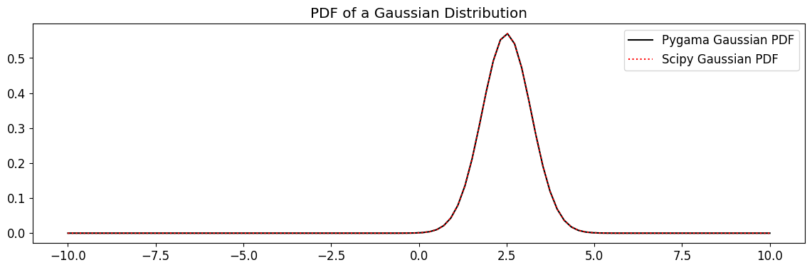
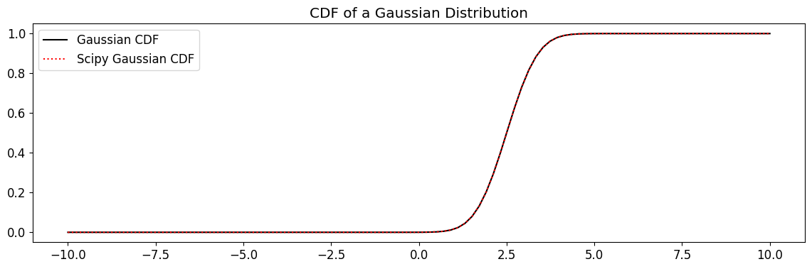
Geez, there are a lot of methods. Let’s hone in on a couple: ### .pdf and .cdf
These are just your bread and butter probability density and cumulative density functions
[3]:
gauss_pdf = gaussian.pdf(x, mu, sigma)

plt.plot(x, gauss_pdf, label="Pygama Gaussian PDF", c="k")
plt.plot(x, norm.pdf(x, mu, sigma), label="Scipy Gaussian PDF", ls=":", alpha=1, c="r")
plt.title("PDF of a Gaussian Distribution")
plt.legend()
plt.show()
[4]:
gauss_cdf = gaussian.cdf(x, mu, sigma)

plt.plot(x, gauss_cdf, label="Gaussian CDF", c="k")
plt.plot(x, norm.cdf(x, mu, sigma), label="Scipy Gaussian CDF", ls=":", alpha=1, c="r")
plt.title("CDF of a Gaussian Distribution")
plt.legend()
plt.show()
Ok, so that’s fine and dandy, what’s so special about a class that reproduces scipy results?
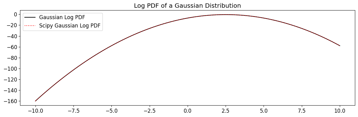
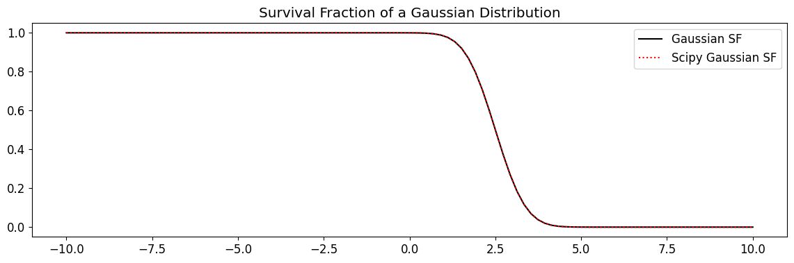
Well, every function in pygama.math.functions subclasses scipy’s rv_continuous class: this allows access to methods that scipy automagically computes. Let’s look at a few
What rv_continuous subclassing gets us: .rvs, .logpdf, .sf…
[5]:
gauss_log_pdf = gaussian.logpdf(x, mu, sigma)

plt.plot(x, gauss_log_pdf, label="Gaussian Log PDF", c="k")
plt.plot(
    x, norm.logpdf(x, mu, sigma), label="Scipy Gaussian Log PDF", ls=":", alpha=1, c="r"
)
plt.title("Log PDF of a Gaussian Distribution")
plt.legend()
plt.show()
[6]:
gauss_sf = gaussian.sf(x, mu, sigma)

plt.plot(x, gauss_sf, label="Gaussian SF", c="k")
plt.plot(x, norm.sf(x, mu, sigma), label="Scipy Gaussian SF", ls=":", alpha=1, c="r")
plt.title("Survival Fraction of a Gaussian Distribution")
plt.legend()
plt.show()
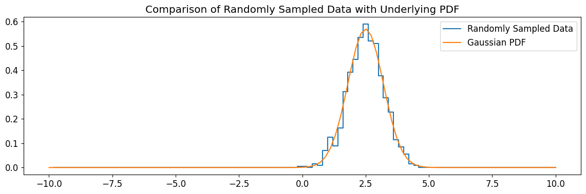
And now for something really useful, random sampling:
[7]:
random_sample = gaussian.rvs(mu, sigma, size=1000, random_state=1)

hist, bins = np.histogram(random_sample, bins=100, range=(-10, 10))
plt.step(
    bins[1:], hist / np.sum(hist) * np.sum(gauss_pdf), label="Randomly Sampled Data"
)
plt.plot(x, gauss_pdf, label="Gaussian PDF")
plt.title("Comparison of Randomly Sampled Data with Underlying PDF")
plt.legend()
plt.show()
We get access to scipy’s rv_continuous methods for free
If we take a look at the actual code for the definition of pygama.math.functions.gaussian we see that there is no direct implementation of methods for .rvs or .logpdf! We get access to all these methods for free. All we have to do is subclass rv_continuous and write definitions for _pdf and _cdf
Now, the drawback: the functions _pdf and _cdf that rv_continuous uses are slow. Let’s see this by comparing to the function that actually computes the pdf: ### But the .pdf and .cdf methods are slow!
[8]:
%%timeit -r 4 -n 10000
gauss_pdf = gaussian.pdf(x, mu, sigma)
35 μs ± 711 ns per loop (mean ± std. dev. of 4 runs, 10,000 loops each)
[9]:
def gaussian_pdf(x, mu, sigma):
    invs = np.inf if sigma == 0 else 1.0 / sigma
    z = (x - mu) * invs
    invnorm = invs / np.sqrt(2 * np.pi)
    return np.exp(-0.5 * z**2) * invnorm
[10]:
%%timeit -r 4 -n 10000
gauss_pdf = gaussian_pdf(x, mu, sigma)
4 μs ± 57.3 ns per loop (mean ± std. dev. of 4 runs, 10,000 loops each)
Fast methods: .get_pdf and .get_cdf
Because the overloaded rv_continuous implementations of pdf and cdf are very slow, we have implemented fast versions of these two methods, named get_pdf and get_cdf.
Each of these fast methods call a numba.njit-wrapped function — a just-in-time compiled function — that runs super fast.
We keep the .pdf and .cdf because they give us access to scipy methods we might want to use, but we write these faster methods so that we can fit distributions quickly.
[11]:
gauss_get_pdf = gaussian.get_pdf(x, mu, sigma)

plt.plot(x, gauss_get_pdf, label="Pygama Gaussian Get_PDF", c="k")
plt.plot(x, norm.pdf(x, mu, sigma), label="Scipy Gaussian PDF", ls=":", alpha=1, c="r")
plt.title("PDF of a Gaussian Distribution")
plt.legend()
plt.show()
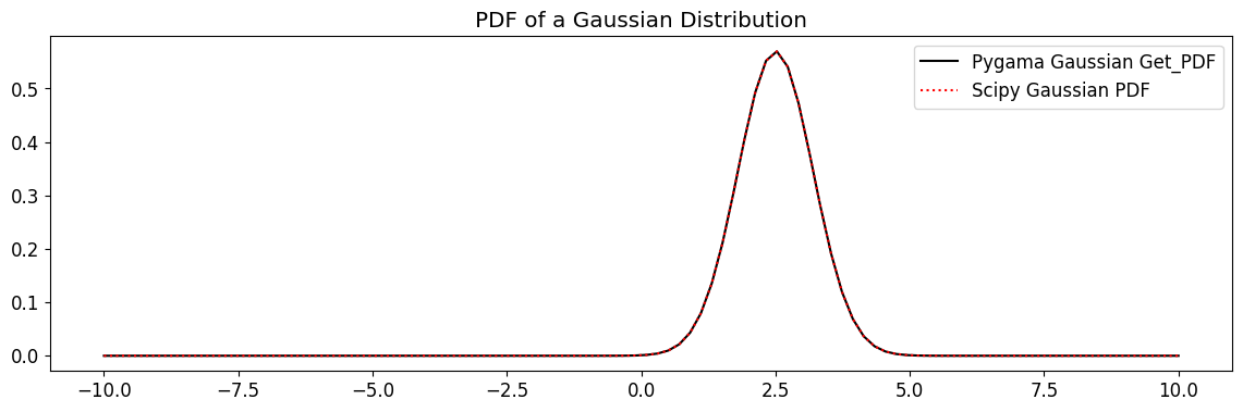
Ok, that’s good that it reproduces the scipy results numerically. But how fast does it run?
[12]:
%%timeit -r 4 -n 10000
gauss_pdf = gaussian.get_pdf(x, mu, sigma)
1.38 μs ± 1.77 ns per loop (mean ± std. dev. of 4 runs, 10,000 loops each)
See, we’re even faster than the function we defined above! That’s the power of just-in-time compiled code
The remaining methods are helpful for binned and unbinned fitting: pdf_norm, cdf_norm, pdf_ext and cdf_ext
For pygama our default way of fitting distributions is to use the Iminuit package. Iminuit has several different ways to fit binned and unbinned data by performing either extended or unextended fits. These fitting methods require functions with different properties. The way pygama functions interact with Iminuit is as follows:
pdf_normis used for unbinned fits, which require a pdf that is normalized to 1 on the fitting rangecdf_normis used for binned fits, which require a cdf that derived from a pdf that is normalized to 1 on the fitting rangepdf_extis used for extended unbinned fits, and the function is required to return a tuple of the support-normalized pdf integrated over the data window, and the scaled support-normalized pdf.cdf_extis used for extended binned fits, and just returns the scaled support-derived cdf
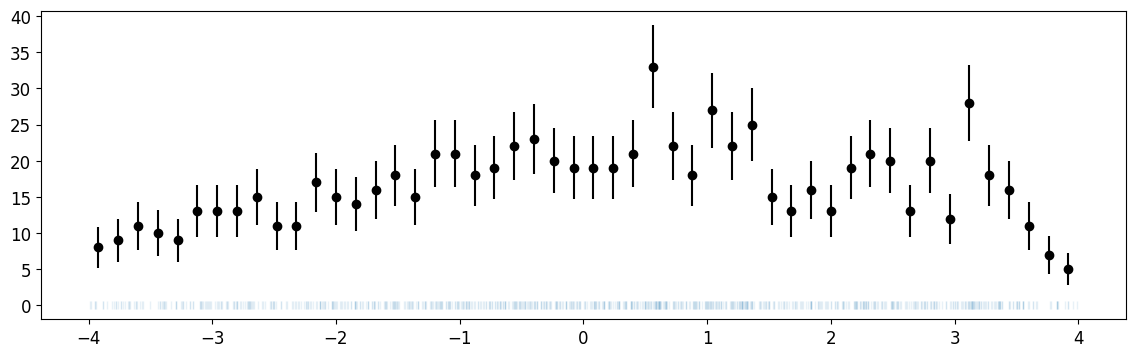
Let’s illustrate some fitting in action, and why some of these weird definitions are required ### Import Iminuit and create data to fit
[13]:
from iminuit import Minuit, cost

xr = (-4, 4)  # xrange
mu = 0.5
sigma = 3

rng = np.random.default_rng(1)

xdata = rng.normal(mu, sigma, size=1000)
xdata = xdata[(xr[0] < xdata) & (xdata < xr[1])]

n, xe = np.histogram(xdata, bins=50, range=xr)
cx = 0.5 * (xe[1:] + xe[:-1])
dx = np.diff(xe)

plt.errorbar(cx, n, n**0.5, fmt="ok")
plt.plot(xdata, np.zeros_like(xdata), "|", alpha=0.1);
Try an unbinned fit using the correct pdf_norm and the incorrect get_pdf
The method pdf_norm requires x_lo, x_hi, which are the bounds of the fitting range, to ensure that the pdf is normalized to unity on. So, every pdf_norm method requires that x_lo and an x_hi are the first two parameters passed to the method call. It’s kind of annoying to feed these parameters to Iminuit and fix them each time, but this results in faster fits over saving x_lo/x_hi as a state inside our method.
We also show a fit with get_pdf to show that the fit returns the incorrect results! We keep the get_pdf methods in pygama because they are useful if we ever need to numerically compute something quickly, or if we do a least squares fit.
[14]:
# Define the cost function
c = cost.UnbinnedNLL(xdata, gaussian.pdf_norm)

m_norm = Minuit(c, x_lo=xr[0], x_hi=xr[1], mu=0.4, sigma=0.2)
m_norm.fixed["x_lo", "x_hi"] = True
m_norm.limits["mu", "sigma"] = (0, None)
m_norm.migrad()
[14]:
| Migrad | |
|---|---|
| FCN = 3418 | Nfcn = 108 |
| EDM = 8.56e-07 (Goal: 0.0002) | time = 1.3 sec |
| Valid Minimum | Below EDM threshold (goal x 10) |
| No parameters at limit | Below call limit |
| Hesse ok | Covariance accurate |
| Name | Value | Hesse Error | Minos Error- | Minos Error+ | Limit- | Limit+ | Fixed | |
|---|---|---|---|---|---|---|---|---|
| 0 | x_lo | -4.00 | 0.04 | yes | ||||
| 1 | x_hi | 4.00 | 0.04 | yes | ||||
| 2 | mu | 0.43 | 0.17 | 0 | ||||
| 3 | sigma | 3.10 | 0.24 | 0 |
| x_lo | x_hi | mu | sigma | |
|---|---|---|---|---|
| x_lo | 0 | 0 | 0.000 | 0.00 |
| x_hi | 0 | 0 | 0.000 | 0.00 |
| mu | 0.000 | 0.000 | 0.0287 | 0.012 (0.300) |
| sigma | 0.00 | 0.00 | 0.012 (0.300) | 0.0569 |
[15]:
c = cost.UnbinnedNLL(xdata, gaussian.get_pdf)

m = Minuit(c, mu=0.4, sigma=0.2)
m.limits["mu", "sigma"] = (0, None)
m.migrad()
[15]:
| Migrad | |
|---|---|
| FCN = 3570 | Nfcn = 90 |
| EDM = 3.38e-06 (Goal: 0.0002) | |
| Valid Minimum | Below EDM threshold (goal x 10) |
| No parameters at limit | Below call limit |
| Hesse ok | Covariance accurate |
| Name | Value | Hesse Error | Minos Error- | Minos Error+ | Limit- | Limit+ | Fixed | |
|---|---|---|---|---|---|---|---|---|
| 0 | mu | 0.19 | 0.07 | 0 | ||||
| 1 | sigma | 2.06 | 0.05 | 0 |
| mu | sigma | |
|---|---|---|
| mu | 0.00508 | 0.0000 |
| sigma | 0.0000 | 0.00254 |
[16]:
plt.errorbar(cx, n, n**0.5, fmt="ok")
xm = np.linspace(*xr)
plt.plot(
    xm, gaussian.pdf_norm(xm, *m_norm.values) * len(xdata) * dx[0], label="pdf_norm fit"
)
plt.plot(xm, gaussian.get_pdf(xm, *m.values) * len(xdata) * dx[0], label="get_pdf fit")
plt.plot(
    xm, gaussian.get_pdf(xm, mu, sigma) * len(xdata) * dx[0], label="True Distribution"
)
plt.legend()
plt.show()
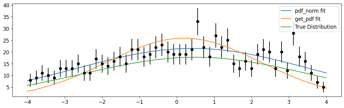
We see that pdf_norm does a much better job of fitting the actual underlying distribution and reproducing the correct \(\mu,\sigma\) parameters
try an extended unbinned fit
The parameters for the pdf_ext are x_lo, x_hi, area, mu, sigma.
[17]:
c = cost.ExtendedUnbinnedNLL(xdata, gaussian.pdf_ext)

m = Minuit(c, x_lo=xr[0], x_hi=xr[1], area=500, mu=0.1, sigma=0.9)
m.fixed["x_lo", "x_hi"] = True
m.limits["area", "mu", "sigma"] = (0, None)
m.migrad()
[17]:
| Migrad | |
|---|---|
| FCN = -6134 | Nfcn = 125 |
| EDM = 9.54e-06 (Goal: 0.0002) | time = 0.2 sec |
| Valid Minimum | Below EDM threshold (goal x 10) |
| No parameters at limit | Below call limit |
| Hesse ok | Covariance accurate |
| Name | Value | Hesse Error | Minos Error- | Minos Error+ | Limit- | Limit+ | Fixed | |
|---|---|---|---|---|---|---|---|---|
| 0 | x_lo | -4.00 | 0.04 | yes | ||||
| 1 | x_hi | 4.00 | 0.04 | yes | ||||
| 2 | area | 1.04e3 | 0.06e3 | 0 | ||||
| 3 | mu | 0.43 | 0.17 | 0 | ||||
| 4 | sigma | 3.10 | 0.24 | 0 |
| x_lo | x_hi | area | mu | sigma | |
|---|---|---|---|---|---|
| x_lo | 0 | 0 | 0 | 0.000 | 0.00 |
| x_hi | 0 | 0 | 0 | 0.000 | 0.00 |
| area | 0 | 0 | 3.42e+03 | 3.024 (0.305) | 10.92 (0.783) |
| mu | 0.000 | 0.000 | 3.024 (0.305) | 0.0287 | 0.012 (0.302) |
| sigma | 0.00 | 0.00 | 10.92 (0.783) | 0.012 (0.302) | 0.0569 |
[18]:
plt.errorbar(cx, n, n**0.5, fmt="ok")
xm = np.linspace(*xr)
plt.plot(xm, gaussian.pdf_ext(xm, *m.values)[1] * dx[0], label="fit")
plt.plot(
    xm, gaussian.pdf_ext(xm, xr[0], xr[1], 1000, mu, sigma)[1] * dx[0], label="actual"
)
plt.legend()
plt.show()
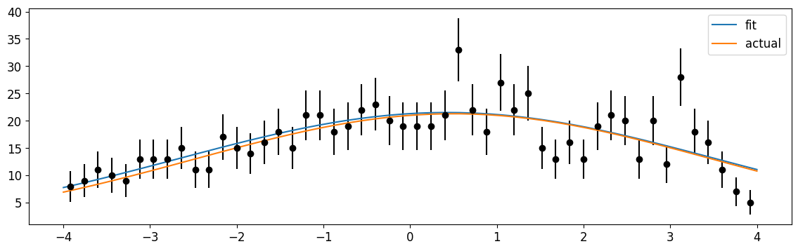
The pdf_ext function correctly fits the area of the curve!
Binned fits using cdf_norm and the incorrect get_cdf
The arguments are in the order x_lo, x_hi, mu, sigma for cdf_norm.
[19]:
c = cost.BinnedNLL(n, xe, gaussian.cdf_norm)

m_norm = Minuit(c, x_lo=xr[0], x_hi=xr[1], mu=0.4, sigma=0.2)
m_norm.fixed["x_lo", "x_hi"] = True
m_norm.limits["mu", "sigma"] = (0.1, None)
m_norm.migrad()
[19]:
| Migrad | |
|---|---|
| FCN = 42.85 (χ²/ndof = 0.9) | Nfcn = 135 |
| EDM = 1.65e-05 (Goal: 0.0002) | time = 2.7 sec |
| Valid Minimum | Below EDM threshold (goal x 10) |
| No parameters at limit | Below call limit |
| Hesse ok | Covariance accurate |
| Name | Value | Hesse Error | Minos Error- | Minos Error+ | Limit- | Limit+ | Fixed | |
|---|---|---|---|---|---|---|---|---|
| 0 | x_lo | -4.00 | 0.04 | yes | ||||
| 1 | x_hi | 4.00 | 0.04 | yes | ||||
| 2 | mu | 0.42 | 0.17 | 0.1 | ||||
| 3 | sigma | 3.08 | 0.23 | 0.1 |
| x_lo | x_hi | mu | sigma | |
|---|---|---|---|---|
| x_lo | 0 | 0 | 0.000 | 0.00 |
| x_hi | 0 | 0 | 0.000 | 0.00 |
| mu | 0.000 | 0.000 | 0.0279 | 0.012 (0.295) |
| sigma | 0.00 | 0.00 | 0.012 (0.295) | 0.0548 |
[20]:
c = cost.BinnedNLL(n, xe, gaussian.get_cdf)

m = Minuit(c, mu=0.4, sigma=0.2)
m.limits["mu", "sigma"] = (0.1, None)
m.migrad()
[20]:
| Migrad | |
|---|---|
| FCN = 193.7 (χ²/ndof = 4.0) | Nfcn = 231 |
| EDM = 5.24e-08 (Goal: 0.0002) | |
| Valid Minimum | Below EDM threshold (goal x 10) |
| No parameters at limit | Below call limit |
| Hesse ok | Covariance accurate |
| Name | Value | Hesse Error | Minos Error- | Minos Error+ | Limit- | Limit+ | Fixed | |
|---|---|---|---|---|---|---|---|---|
| 0 | mu | 0.19 | 0.07 | 0.1 | ||||
| 1 | sigma | 2.05 | 0.05 | 0.1 |
| mu | sigma | |
|---|---|---|
| mu | 0.00506 | 0.0000 |
| sigma | 0.0000 | 0.00253 |
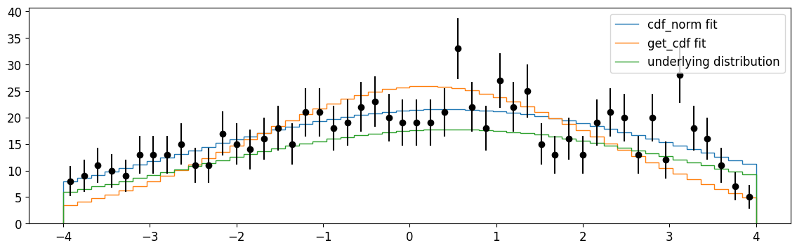
[21]:
plt.errorbar(cx, n, n**0.5, fmt="ok")
plt.stairs(
    np.diff(gaussian.cdf_norm(xe, *m_norm.values)) * len(xdata),
    xe,
    label="cdf_norm fit",
)
plt.stairs(
    np.diff(gaussian.get_cdf(xe, *m.values)) * len(xdata), xe, label="get_cdf fit"
)
plt.stairs(
    np.diff(gaussian.get_cdf(xe, mu, sigma)) * len(xdata),
    xe,
    label="underlying distribution",
)
plt.legend()
plt.show()
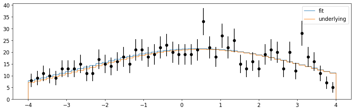
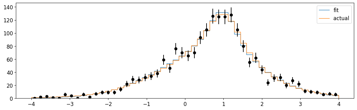
Finally, extended binned fits with cdf_ext
[22]:
c = cost.ExtendedBinnedNLL(n, xe, gaussian.cdf_ext)

m = Minuit(c, area=500, mu=0.1, sigma=0.9)
m.limits["area", "mu", "sigma"] = (0, None)
m.migrad()
[22]:
| Migrad | |
|---|---|
| FCN = 42.85 (χ²/ndof = 0.9) | Nfcn = 128 |
| EDM = 4.11e-06 (Goal: 0.0002) | time = 0.5 sec |
| Valid Minimum | Below EDM threshold (goal x 10) |
| No parameters at limit | Below call limit |
| Hesse ok | Covariance accurate |
| Name | Value | Hesse Error | Minos Error- | Minos Error+ | Limit- | Limit+ | Fixed | |
|---|---|---|---|---|---|---|---|---|
| 0 | area | 1.04e3 | 0.06e3 | 0 | ||||
| 1 | mu | 0.42 | 0.17 | 0 | ||||
| 2 | sigma | 3.08 | 0.23 | 0 |
| area | mu | sigma | |
|---|---|---|---|
| area | 3.3e+03 | 2.845 (0.297) | 10.42 (0.776) |
| mu | 2.845 (0.297) | 0.0279 | 0.012 (0.295) |
| sigma | 10.42 (0.776) | 0.012 (0.295) | 0.0547 |
[23]:
plt.errorbar(cx, n, n**0.5, fmt="ok")
plt.stairs(np.diff(gaussian.cdf_ext(xe, *m.values)), xe, label="fit")
plt.stairs(np.diff(gaussian.cdf_ext(xe, 1000, mu, sigma)), xe, label="underlying")
plt.legend();
Writing our own pygama.math distribution: conventions and requirements
Let’s write a Cauchy distribution. Recall that a Cauchy distribution has support over the real line, and has a pdf like
\(pdf(x, \mu,\sigma) = \frac{1}{\pi\sigma\left[1+\left(\frac{x-\mu}{\sigma}\right)^2\right]}\)
and a cdf:
\(cdf(x, \mu,\sigma) = \frac{1}{\pi}\arctan\left(\frac{x-\mu}{\sigma}\right)+\frac{1}{2}\)
What we need to define a distribution class
We need four functions that our class methods will call and their arguments, and they all should be numbafied
A PDF, normalized to the support. Args: x, mu, sigma
A CDF, derived from the support normalized PDF. Args: x, mu, sigma
A scaled PDF. Args: x, area, mu, sigma
A scaled CDF. Args: x, area, mu, sigma
The convention is to name these functions nb_distribution_pdf and nb_distribution_scaled_cdf for example.
[24]:
import numba as nb

# here we set some parameters to ensure that numba will compute things as quickly as possible
kwd_parallel = {"parallel": True, "fastmath": True}
kwd = {"parallel": False, "fastmath": True}


# define the pdf
@nb.njit(**kwd_parallel)
def nb_cauchy_pdf(x: np.ndarray, mu: float, sigma: float) -> np.ndarray:
    r"""
    Parameters
    ----------
    x
        The input data
    lamb
        The rate
    mu
        The amount to shift the distribution
    sigma
        The amount to scale the distribution
    """

    y = np.empty_like(x, dtype=np.float64)
    # we want to do a loop because it is faster with parallelization
    for i in nb.prange(x.shape[0]):
        y[i] = (x[i] - mu) / sigma
        y[i] = 1 / (np.pi * sigma * (1 + y[i] ** 2))
    return y


# define the cdf
@nb.njit(**kwd_parallel)
def nb_cauchy_cdf(x: np.ndarray, mu: float, sigma: float) -> np.ndarray:
    r"""
    Parameters
    ----------
    x
        The input data
    lamb
        The rate
    mu
        The amount to shift the distribution
    sigma
        The amount to scale the distribution
    """
    y = np.empty_like(x, dtype=np.float64)
    for i in nb.prange(x.shape[0]):
        y[i] = (x[i] - mu) / sigma
        y[i] = (1 / np.pi) * np.arctan(y[i]) + 0.5
    return y


# define the scaled pdf, can't use parallelization here because there is no outer for-loop
@nb.njit(**kwd)
def nb_cauchy_scaled_pdf(
    x: np.ndarray, area: float, mu: float, sigma: float
) -> np.ndarray:
    r"""
    Parameters
    ----------
    x
        The input data
    area
        The prefactor to scale the pdf by
    lamb
        The rate
    mu
        The amount to shift the distribution
    sigma
        The amount to scale the distribution
    """
    return area * nb_cauchy_pdf(x, mu, sigma)


# define the scaled cdf, can't use parallelization here because there is no outer for-loop
@nb.njit(**kwd)
def nb_cauchy_scaled_cdf(
    x: np.ndarray, area: float, mu: float, sigma: float
) -> np.ndarray:
    r"""
    Parameters
    ----------
    x
        The input data
    area
        The prefactor to scale the pdf by
    lamb
        The rate
    mu
        The amount to shift the distribution
    sigma
        The amount to scale the distribution
    """
    return area * nb_cauchy_cdf(x, mu, sigma)
Now we create a class using these four functions
Each pygama distribution class subclasses pygama_continuous, which itself is a subclass of rv_continuous.
An aside on the ordering of parameters:
In the following the term “shape parameter” refers to a specific variable used to define a distribution that is not an overall scaling (which I call \(\mu\)) or shifting (which I call \(\sigma\)). An example of shape parameters would be the \(\beta, m\) parameters in a crystal ball function. The location and scale (\(\mu, \sigma\)) parameters have a more specific definition — akin to what scipy does. If a \(\mu, \sigma\) value is present, then the entire distribution is
shifted and scaled; this can be achieved by transforming \(y = \frac{x-\mu}{\sigma}\) and computing \(pdf(y)/\sigma\) ( where the factor of \(1/\sigma\) comes from the Jacobian).
The ordering of parameters is as follows, using whichever are needed for a function: x, x_lo, x_hi, area, mu, sigma, shapes, ...
Where x_lo and x_hi are the lower and upper bounds to evaluate a function on. These are particularly important when the support of a function depends on its fit range; distributions like uniform, linear, and step distributions are defined on a finite support and thus x_lo and x_hi are parameters that should be passed to every function call.
Now, back to require methods
The class name has the format distribution_name_gen and it must include the following methods with their arguments:
_pdf(self, x, mu, sigma, shapes):This is an overloading of the
scipymethod for the pdf. If shape parameters are present,nb_distribution_pdfmust also be called withshape_param[0]becausescipypasses an array of shape parameters to the function calls. Finally,x.flags.writeable = Truemust be passed so thatnumbacan operate as expected on arrays._cdf(self, x, mu, sigma, shapes):This is an overloading of the
scipymethod for the cdf. The same format applies as for the pdf.get_pdf(x, mu, sigma, shapes):This is a direct call to the fast
nb_distribution_pdfget_pdf(x, mu, sigma, shapes):This is a direct call to the fast
nb_distribution_cdfpdf_norm(x, x_lo, x_hi, mu, sigma, shapes):In the case that the support of the distribution is the entire real line, this calls a
pygama_continuoussuper method that normalizes the pdf to unity on the range \([x_{lo},x_{hi}]\) by computing \(\frac{pdf(x)}{cdf(x_{hi})- cdf(x_{lo})}\). If the distribution is defined on a limited domain, this function needs to be directly overloaded – seepygama.math.functions.stepfor an example.cdf_norm(x, x_lo, x_hi, mu, sigma, shapes):In the case that the support of the distribution is the entire real line, this calls a
pygama_continuoussuper method that derives the cdf from a pdf that is normalized to unity on the range \([x_{lo},x_{hi}]\) by computing \(\frac{cdf(x)}{cdf(x_{hi})- cdf(x_{lo})}\). If the distribution is defined on a limited domain, this function needs to be directly overloaded – seepygama.math.functions.stepfor an example.pdf_ext(x, x_lo, x_hi, area, mu, sigma, shapes):A function that returns both the integral of the support-normalized pdf on the interval \([x_{lo},x_{hi}]\), as well as the support-normalized pdf on that range as well. The fastest way to compute these is to return
np.diff(nb_distribution_scaled_cdf(np.array([x_lo, x_hi]), area, mu, sigma, shapes))andnb_distribution_scaled_pdf(x, area, mu, sigma, shapes)cdf_ext(x, area, mu, sigma, shapes):A function that returns just the scaled cdf,
nb_distribution_scaled_cdf(x, area, mu, sigma, shapes)req_args(self):A function that returns a tuple with the strings of the names of the required shape parameters and mu and sigma
[25]:
from pygama.math.functions.pygama_continuous import PygamaContinuous


class cauchy_gen(PygamaContinuous):
    def _pdf(self, x: np.ndarray) -> np.ndarray:
        x.flags.writeable = True
        return nb_cauchy_pdf(x, 0, 1)

    def _cdf(self, x: np.ndarray) -> np.ndarray:
        x.flags.writeable = True
        return nb_cauchy_cdf(x, 0, 1)

    def get_pdf(self, x: np.ndarray, mu: float, sigma: float) -> np.ndarray:
        return nb_cauchy_pdf(x, mu, sigma)

    def get_cdf(self, x: np.ndarray, mu: float, sigma: float) -> np.ndarray:
        return nb_cauchy_cdf(x, mu, sigma)

    # needed so that we can hack iminuit's introspection to function parameter names.
    def pdf_norm(
        self, x: np.ndarray, x_lo: float, x_hi: float, mu: float, sigma: float
    ) -> np.ndarray:
        return self._pdf_norm(x, x_lo, x_hi, mu, sigma)

    def cdf_norm(
        self, x: np.ndarray, x_lo: float, x_hi: float, mu: float, sigma: float
    ) -> np.ndarray:
        return self._cdf_norm(x, x_lo, x_hi, mu, sigma)

    def pdf_ext(
        self,
        x: np.ndarray,
        x_lo: float,
        x_hi: float,
        area: float,
        mu: float,
        sigma: float,
    ) -> np.ndarray:
        return np.diff(nb_cauchy_scaled_cdf(np.array([x_lo, x_hi]), area, mu, sigma))[
            0
        ], nb_cauchy_scaled_pdf(x, area, mu, sigma)

    def cdf_ext(
        self, x: np.ndarray, area: float, mu: float, sigma: float
    ) -> np.ndarray:
        return nb_cauchy_scaled_cdf(x, area, mu, sigma)

    def required_args(self) -> tuple[str, str]:
        return "mu", "sigma"


cauchy = cauchy_gen(name="cauchy")
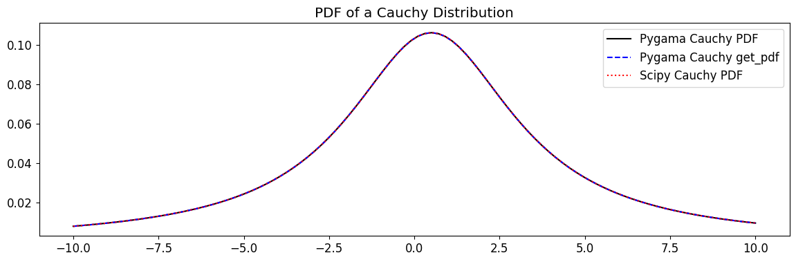
[26]:
from scipy.stats import cauchy as scipy_cauchy
cauchy_pdf = cauchy.pdf(x, mu, sigma)
cauchy_get_pdf = cauchy.get_pdf(x, mu, sigma)
cauchy_cdf = cauchy.cdf(x, mu, sigma)
cauchy_get_cdf = cauchy.get_cdf(x, mu, sigma)
plt.plot(x, cauchy_pdf, label="Pygama Cauchy PDF", c="k")
plt.plot(x, cauchy_get_pdf, label="Pygama Cauchy get_pdf", c="b", ls="--")
plt.plot(
x, scipy_cauchy.pdf(x, mu, sigma), label="Scipy Cauchy PDF", ls=":", alpha=1, c="r"
)
plt.title("PDF of a Cauchy Distribution")
plt.legend()
plt.show()
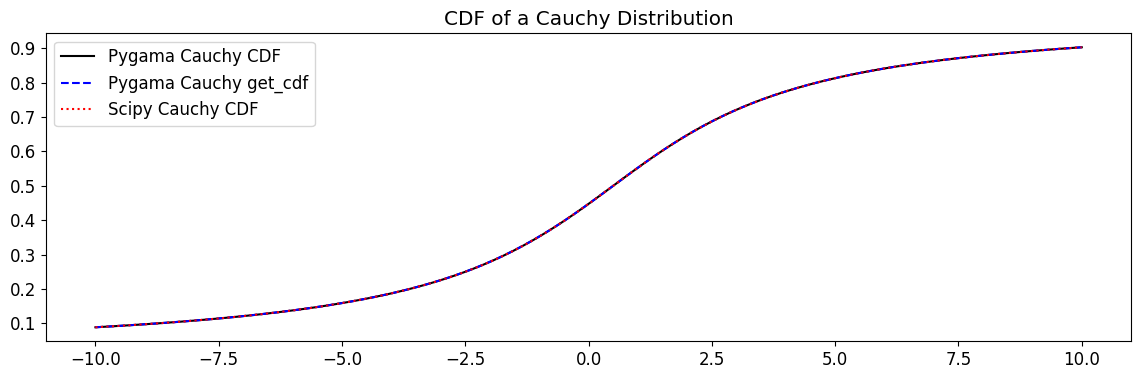
plt.plot(x, cauchy_cdf, label="Pygama Cauchy CDF", c="k")
plt.plot(x, cauchy_get_cdf, label="Pygama Cauchy get_cdf", c="b", ls="--")
plt.plot(
x, scipy_cauchy.cdf(x, mu, sigma), label="Scipy Cauchy CDF", ls=":", alpha=1, c="r"
)
plt.title("CDF of a Cauchy Distribution")
plt.legend()
plt.show()
Perform some fits using the new Cauchy distribution to show the other methods’ validity
[27]:
xr = (-4, 4) # xrange
mu = 0.5
sigma = 0.7
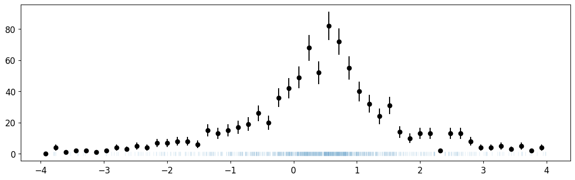
xdata = scipy_cauchy.rvs(mu, sigma, size=1000, random_state=42)
xdata = xdata[(xr[0] < xdata) & (xdata < xr[1])]
n, xe = np.histogram(xdata, bins=50, range=xr)
cx = 0.5 * (xe[1:] + xe[:-1])
dx = np.diff(xe)
plt.errorbar(cx, n, n**0.5, fmt="ok")
plt.plot(xdata, np.zeros_like(xdata), "|", alpha=0.1);
unbinned fit
[28]:
c = cost.UnbinnedNLL(xdata, cauchy.pdf_norm)

m_norm = Minuit(c, x_lo=xr[0], x_hi=xr[1], mu=0.4, sigma=0.2)
m_norm.fixed["x_lo", "x_hi"] = True
m_norm.limits["mu", "sigma"] = (0, None)
m_norm.migrad()
[28]:
| Migrad | |
|---|---|
| FCN = 2784 | Nfcn = 56 |
| EDM = 1.66e-07 (Goal: 0.0002) | time = 0.4 sec |
| Valid Minimum | Below EDM threshold (goal x 10) |
| No parameters at limit | Below call limit |
| Hesse ok | Covariance accurate |
| Name | Value | Hesse Error | Minos Error- | Minos Error+ | Limit- | Limit+ | Fixed | |
|---|---|---|---|---|---|---|---|---|
| 0 | x_lo | -4.00 | 0.04 | yes | ||||
| 1 | x_hi | 4.00 | 0.04 | yes | ||||
| 2 | mu | 0.478 | 0.033 | 0 | ||||
| 3 | sigma | 0.73 | 0.04 | 0 |
| x_lo | x_hi | mu | sigma | |
|---|---|---|---|---|
| x_lo | 0 | 0 | 0.0000 | 0.0000 |
| x_hi | 0 | 0 | 0.0000 | 0.0000 |
| mu | 0.0000 | 0.0000 | 0.00106 | -0.0000 (-0.018) |
| sigma | 0.0000 | 0.0000 | -0.0000 (-0.018) | 0.00147 |
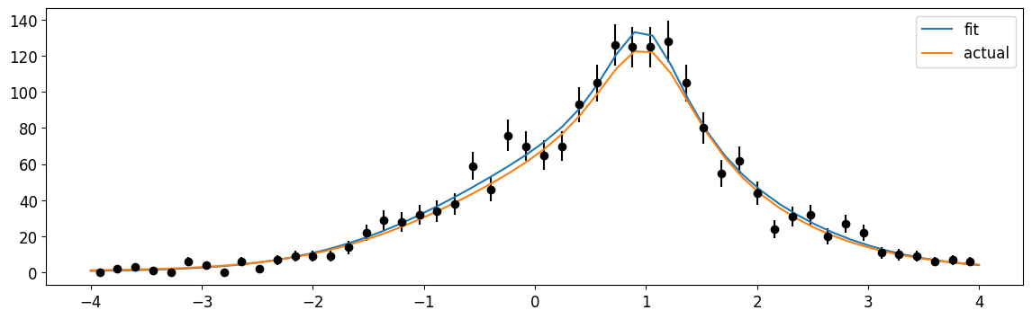
extended unbinned fit
[29]:
c = cost.ExtendedUnbinnedNLL(xdata, cauchy.pdf_ext)

m = Minuit(c, x_lo=xr[0], x_hi=xr[1], area=500, mu=0.1, sigma=0.9)
m.fixed["x_lo", "x_hi"] = True
m.limits["area", "mu", "sigma"] = (0.01, None)
m.migrad()
[29]:
| Migrad | |
|---|---|
| FCN = -7457 | Nfcn = 102 |
| EDM = 2.22e-07 (Goal: 0.0002) | time = 0.2 sec |
| Valid Minimum | Below EDM threshold (goal x 10) |
| No parameters at limit | Below call limit |
| Hesse ok | Covariance accurate |
| Name | Value | Hesse Error | Minos Error- | Minos Error+ | Limit- | Limit+ | Fixed | |
|---|---|---|---|---|---|---|---|---|
| 0 | x_lo | -4.00 | 0.04 | yes | ||||
| 1 | x_hi | 4.00 | 0.04 | yes | ||||
| 2 | area | 1.002e3 | 0.034e3 | 0.01 | ||||
| 3 | mu | 0.478 | 0.033 | 0.01 | ||||
| 4 | sigma | 0.73 | 0.04 | 0.01 |
| x_lo | x_hi | area | mu | sigma | |
|---|---|---|---|---|---|
| x_lo | 0 | 0 | 0 | 0.0000 | 0.0000 |
| x_hi | 0 | 0 | 0 | 0.0000 | 0.0000 |
| area | 0 | 0 | 1.18e+03 | 0.0042 | 0.2596 (0.197) |
| mu | 0.0000 | 0.0000 | 0.0042 | 0.00106 | -0.0000 (-0.018) |
| sigma | 0.0000 | 0.0000 | 0.2596 (0.197) | -0.0000 (-0.018) | 0.00147 |
Binned fit
[30]:
c = cost.BinnedNLL(n, xe, cauchy.cdf_norm)

m_norm = Minuit(c, x_lo=xr[0], x_hi=xr[1], mu=0.4, sigma=0.2)
m_norm.fixed["x_lo", "x_hi"] = True
m_norm.limits["mu", "sigma"] = (0.1, None)
m_norm.migrad()
[30]:
| Migrad | |
|---|---|
| FCN = 52.27 (χ²/ndof = 1.1) | Nfcn = 48 |
| EDM = 3.04e-05 (Goal: 0.0002) | |
| Valid Minimum | Below EDM threshold (goal x 10) |
| No parameters at limit | Below call limit |
| Hesse ok | Covariance accurate |
| Name | Value | Hesse Error | Minos Error- | Minos Error+ | Limit- | Limit+ | Fixed | |
|---|---|---|---|---|---|---|---|---|
| 0 | x_lo | -4.00 | 0.04 | yes | ||||
| 1 | x_hi | 4.00 | 0.04 | yes | ||||
| 2 | mu | 0.482 | 0.033 | 0.1 | ||||
| 3 | sigma | 0.73 | 0.04 | 0.1 |
| x_lo | x_hi | mu | sigma | |
|---|---|---|---|---|
| x_lo | 0 | 0 | 0.0000 | 0.0000 |
| x_hi | 0 | 0 | 0.0000 | 0.0000 |
| mu | 0.0000 | 0.0000 | 0.00107 | -0.0000 (-0.024) |
| sigma | 0.0000 | 0.0000 | -0.0000 (-0.024) | 0.00149 |
Extended binned fit
[31]:
c = cost.ExtendedBinnedNLL(n, xe, cauchy.cdf_ext)

m = Minuit(c, area=500, mu=0.1, sigma=0.9)
m.limits["area", "mu", "sigma"] = (0, None)
m.migrad()
[31]:
| Migrad | |
|---|---|
| FCN = 52.27 (χ²/ndof = 1.1) | Nfcn = 95 |
| EDM = 6.18e-06 (Goal: 0.0002) | |
| Valid Minimum | Below EDM threshold (goal x 10) |
| No parameters at limit | Below call limit |
| Hesse ok | Covariance accurate |
| Name | Value | Hesse Error | Minos Error- | Minos Error+ | Limit- | Limit+ | Fixed | |
|---|---|---|---|---|---|---|---|---|
| 0 | area | 1.002e3 | 0.034e3 | 0 | ||||
| 1 | mu | 0.483 | 0.033 | 0 | ||||
| 2 | sigma | 0.73 | 0.04 | 0 |
| area | mu | sigma | |
|---|---|---|---|
| area | 1.18e+03 | 0.0030 | 0.2636 (0.199) |
| mu | 0.0030 | 0.00107 | -0.0000 (-0.024) |
| sigma | 0.2636 (0.199) | -0.0000 (-0.024) | 0.00149 |
Adding distributions with SumDists
In the business of fitting data, adding two distributions together is our bread-and-butter. This part of the notebook will show you how to create your own distribution that is an instance of pygama.math.sum_dists. There are a couple of different use cases for adding distributions together, and we will look at each in turn, but here is a summary:
Adding different fractions of distributions together, and fitting out the relative amount of distributions
Adding distributions with different areas (present in equal fractions) and fitting the areas
Let’s first create the synthetic data that we will fit
[32]:
xr = (-4, 4) # xrange
rng = np.random.default_rng(1)
mu = 0.5
sigma = 1.3
mu2 = 1
sigma2 = 0.6
xdata = norm.rvs(mu, sigma, size=1000, random_state=42)
ydata = scipy_cauchy.rvs(mu2, sigma2, size=len(xdata), random_state=42)
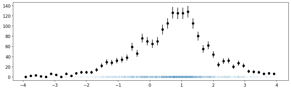
xmix = np.append(xdata, ydata)
xmix = xmix[(xr[0] < xmix) & (xmix < xr[1])]
n, xe = np.histogram(xmix, bins=50, range=xr)
cx = 0.5 * (xe[1:] + xe[:-1])
dx = np.diff(xe)
plt.errorbar(cx, n, n**0.5, fmt="ok")
plt.plot(xmix, np.zeros_like(xmix), "|", alpha=0.1);
A little about SumDists
The first important thing to note about this class is that all methods in this class are of the form method(x, *parameter_array) or method(x, parameters, ...).
SumDists works by adding two — and only two — distributions together. The first thing a user does in creating a new instance is define the order of elements in a parameter_array. Then, sum_dists works by grabbing elements at different indices in this parameter_array according to rules that the user provides in the instantiation. Here’s how to write a generic class:
Create a
parameter_index_arraythat holds the indices of what will eventually come in theparameter_array. If the user will eventually passparameters = [frac1, mu, sigma]then we just takeparameter_index_array=[frac1, mu, sigma]=range(3)SumDiststakes an alternating pattern of distributions and distribution-specific parameter_index_arrays. Each par array can contain[mu, sigma, shape]. These par arrays are placed in a tuple with their distribution like(dist1, [mu1, sigma1, shape1]). Finally, a list of these tuples is fed to the constructor assum_dists([(dist1, [mu1, sigma1, shape1]), (dist2, [mu2, sigma2])])The
SumDistsconstructor then takes an array corresponding the index locations of where either fraction or area values will be passed in the ultimateparameter_index_array.We pass one of the 4 flag options, to be described below.
We can optionally pass a list of parameter names, but these can also be calculated automatically if left as None
Let’s trace through how the code works for a simple example. Suppose we want to create the following distribution
\(new\_pdf(x, \mu, \sigma, \tau, frac_1) = frac_1\cdot dist_1(x, \mu, \sigma, \tau) + (1-frac1)\cdot dist_2(x, \mu, \sigma)\)
The first thing we would do is create our parameter_index_array
[mu, sigma, tau, frac_1] = range(4)
Then, we would create our alternating pattern of distributions and parameter index arrays:
args = [(dist1, [mu, sigma, tau]), (dist2, [mu, sigma])]
Finally, we would initialize (with the fracs flag in this case, more on that later)
SumDists(args, area_frac_idxs = [frac_1], frac_flag = "fracs", parameter_names=["mu", "sigma", "tau", "frac_1"])
So… What is SumDists actually doing?
Under the hood, SumDists is applying a set of rules so that the following is always computed, regardless of the flag sent to the constructor.
area1*frac1*dist1(x, mu, sigma, shape) + area2*frac2*dist_2(x, mu2, sigma2, shape2)
It computes this by first grabbing the relevant areas or fraction values from their position in the parameter_index_array. Then, at the time of method call, SumDists grabs the values from parameter_index_array that correspond to each distribution via slicing the parameter_index_array with the individual par arrays passed in the instantiation. In our example above, SumDists knows to grab the values at indices 0, 1, 2 for the first distribution because it is instantiated with
the tuple (dist1, [mu, sigma, tau]).
There’s also some work done to determine which of area and frac are present. That’s the purpose of the flag. Let’s take some time and learn a little more about what each flag does.
The flag in the SumDists constructor
Let’s say we are interested in knowing the amount of counts present in a signal and a background in our total spectrum, i.e. we want to create and fit a function that looks like
\(pdf= A\cdot gauss\_pdf + B\cdot cauchy\_pdf\)
Because we are interested in fitting the areas, we send the areas keyword to flag. This causes SumDists to look for an area_frac_idxs array of length 2 in the instantiation: this array contains the indices that the area values will be located at in the parameter_index_array. The areas keyword causes the fractions to be set to 1.
In our example above for constructing \(new\_pdf(x, \mu, \sigma, \tau, frac_1) = frac_1\cdot dist_1(x, \mu, \sigma, \tau) + (1-frac1)\cdot dist_2(x, \mu, \sigma)\), the instantiation takes the fracs keyword. This causes sum_dists to look for an area_frac_idxs array of length 1 in the instantiation: this array contains the index that the fraction values will be located at in the parameter_index_array. sum_dists works by multiplying frac times the first distribution,
and 1-frac times the second distribution.
An aside on conventions
The ultimate parameter_index_array that the user passes to the methods should look like x_lo, x_hi, area/frac_1, mu, sigma, shapes1, area/frac2, mu2, sigma2, shapes2 based on which are present. For distributions with ill-defined support, such as a step or linear function, the user must always pass x_lo, x_hi for every method call such as gauss_on_step.get_pdf. If a sum_dists instance is created from distributions with well-defined support, then sum_dist requires that for
pdf_norm, cdf_norm, pdf_ext that x_lo, x_hi are added at the front of the parameter index array; for ill-defined distributions it knows to look for x_lo, x_hi at the user specified location. This means that for pdf_norm, cdf_norm, pdf_ext the fit/normalization range is always set equal to the support range.
[33]:
from pygama.math.functions.sum_dists import SumDists

# we first create an array contains the indices of the parameter array
# that will eventually be input to function calls
(area1, mu, sigma, area2, mu2, sigma2) = range(6)

# we now create an array containing the tuples of the distributions and their shape parameters
args = [(gaussian, [mu, sigma]), (cauchy, [mu2, sigma2])]
# we initialize with the flag = "areas" to let the constructor know we are sending area parameter idxs only
cauchy_on_gauss = SumDists(
    args,
    area_frac_idxs=[area1, area2],
    flag="areas",
    parameter_names=["area1", "mu", "sigma", "area2", "mu2", "sigma2"],
)
That was super quick, let’s see how it does with fitting data
Because we are interested in fitting out areas, we need to use the extended forms of our fits And for pdf_ext we need to pass x_lo, x_hi as the first two values, and fix them before fitting.
[34]:
c = cost.ExtendedUnbinnedNLL(xmix, cauchy_on_gauss.pdf_ext)

m = Minuit(c, xr[0], xr[1], 1000, 0.5, 1.3, 1000, 1, 2)
m.fixed[0, 1] = True
m.limits[2, 5] = (0, None)
m.limits[3, 5, 6, 7] = (0, 2)
print(m.migrad())


plt.errorbar(cx, n, n**0.5, fmt="ok")
xm = np.linspace(*xr)
plt.plot(xm, cauchy_on_gauss.pdf_ext(xm, *m.values)[1] * dx[0], label="fit")
plt.plot(
    xm,
    cauchy_on_gauss.pdf_ext(xm, xr[0], xr[1], 1000, 0.5, 1.3, 1000, 1, 0.6)[1] * dx[0],
    label="actual",
)
plt.legend();
┌─────────────────────────────────────────────────────────────────────────┐
│                                Migrad                                   │
├──────────────────────────────────┬──────────────────────────────────────┤
│ FCN = -1.866e+04                 │              Nfcn = 362              │
│ EDM = 2.38e-05 (Goal: 0.0002)    │                                      │
├──────────────────────────────────┼──────────────────────────────────────┤
│          Valid Minimum           │   Below EDM threshold (goal x 10)    │
├──────────────────────────────────┼──────────────────────────────────────┤
│     SOME parameters at limit     │           Below call limit           │
├──────────────────────────────────┼──────────────────────────────────────┤
│             Hesse ok             │         Covariance accurate          │
└──────────────────────────────────┴──────────────────────────────────────┘
┌───┬────────┬───────────┬───────────┬────────────┬────────────┬─────────┬─────────┬───────┐
│   │ Name   │   Value   │ Hesse Err │ Minos Err- │ Minos Err+ │ Limit-  │ Limit+  │ Fixed │
├───┼────────┼───────────┼───────────┼────────────┼────────────┼─────────┼─────────┼───────┤
│ 0 │ x_lo   │   -4.00   │   0.04    │            │            │         │         │  yes  │
│ 1 │ x_hi   │   4.00    │   0.04    │            │            │         │         │  yes  │
│ 2 │ area1  │  1.90e3   │  0.04e3   │            │            │    0    │         │       │
│ 3 │ mu     │   0.696   │   0.029   │            │            │    0    │    2    │       │
│ 4 │ sigma  │   1.251   │   0.022   │            │            │         │         │       │
│ 5 │ area2  │    2.0    │    1.9    │            │            │    0    │    2    │       │
│ 6 │ mu2    │ 990.45e-3 │  0.12e-3  │            │            │    0    │    2    │       │
│ 7 │ sigma2 │  0.08e-3  │  0.08e-3  │            │            │    0    │    2    │       │
└───┴────────┴───────────┴───────────┴────────────┴────────────┴─────────┴─────────┴───────┘
┌────────┬─────────────────────────────────────────────────────────────────────────────────────────┐
│        │       x_lo       x_hi      area1         mu      sigma      area2        mu2     sigma2 │
├────────┼─────────────────────────────────────────────────────────────────────────────────────────┤
│   x_lo │          0          0          0          0          0          0          0       0e-9 │
│   x_hi │          0          0          0          0          0          0          0       0e-9 │
│  area1 │          0          0   1.91e+03    18.2e-3    25.4e-3  -28.56e-6  14.267e-6 -27.529e-6 │
│     mu │          0          0    18.2e-3   0.000861          0         -0   0.002e-6      -4e-9 │
│  sigma │          0          0    25.4e-3          0   0.000484    0.01e-6  -0.005e-6      10e-9 │
│  area2 │          0          0  -28.56e-6         -0    0.01e-6   1.37e-07  -0.001e-6       1e-9 │
│    mu2 │          0          0  14.267e-6   0.002e-6  -0.005e-6  -0.001e-6   1.31e-08      -4e-9 │
│ sigma2 │       0e-9       0e-9 -27.529e-6      -4e-9      10e-9       1e-9      -4e-9   5.73e-09 │
└────────┴─────────────────────────────────────────────────────────────────────────────────────────┘
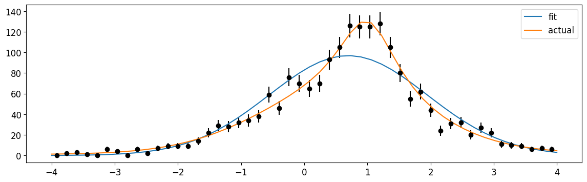
Well, that’s pretty good! Let’s see how the extended unbinned fit fairs
[35]:
c = cost.ExtendedBinnedNLL(n, xe, cauchy_on_gauss.cdf_ext)
m = Minuit(c, 100, 0.1, 0.3, 100, 1, 2)
m.limits[0, 3] = (0, None)
m.limits[1, 2, 4, 5] = (0, 2)
print(m.migrad())

plt.errorbar(cx, n, n**0.5, fmt="ok")
plt.stairs(np.diff(cauchy_on_gauss.cdf_ext(xe, *np.array(m.values))), xe, label="fit")
plt.stairs(
    np.diff(cauchy_on_gauss.cdf_ext(xe, *np.array([1000, 0.5, 1.3, 1000, 1, 0.6]))),
    xe,
    label="actual",
)
plt.legend();
┌─────────────────────────────────────────────────────────────────────────┐
│                                Migrad                                   │
├──────────────────────────────────┬──────────────────────────────────────┤
│ FCN = 58.66 (χ²/ndof = 1.3)      │              Nfcn = 461              │
│ EDM = 9.18e-05 (Goal: 0.0002)    │                                      │
├──────────────────────────────────┼──────────────────────────────────────┤
│          Valid Minimum           │   Below EDM threshold (goal x 10)    │
├──────────────────────────────────┼──────────────────────────────────────┤
│      No parameters at limit      │           Below call limit           │
├──────────────────────────────────┼──────────────────────────────────────┤
│             Hesse ok             │         Covariance accurate          │
└──────────────────────────────────┴──────────────────────────────────────┘
┌───┬────────┬───────────┬───────────┬────────────┬────────────┬─────────┬─────────┬───────┐
│   │ Name   │   Value   │ Hesse Err │ Minos Err- │ Minos Err+ │ Limit-  │ Limit+  │ Fixed │
├───┼────────┼───────────┼───────────┼────────────┼────────────┼─────────┼─────────┼───────┤
│ 0 │ area1  │  1.20e3   │  0.14e3   │            │            │    0    │         │       │
│ 1 │ mu     │   0.57    │   0.06    │            │            │    0    │    2    │       │
│ 2 │ sigma  │   1.32    │   0.05    │            │            │    0    │    2    │       │
│ 3 │ area2  │  0.77e3   │  0.15e3   │            │            │    0    │         │       │
│ 4 │ mu2    │   0.98    │   0.05    │            │            │    0    │    2    │       │
│ 5 │ sigma2 │   0.49    │   0.08    │            │            │    0    │    2    │       │
└───┴────────┴───────────┴───────────┴────────────┴────────────┴─────────┴─────────┴───────┘
┌────────┬───────────────────────────────────────────────────────┐
│        │    area1       mu    sigma    area2      mu2   sigma2 │
├────────┼───────────────────────────────────────────────────────┤
│  area1 │ 1.82e+04    4.662   1.4760 -0.020e6   0.6312   -9.059 │
│     mu │    4.662  0.00388   0.0007   -5.312  -0.0009   -0.002 │
│  sigma │   1.4760   0.0007  0.00208  -1.7600  -0.0004  -0.0018 │
│  area2 │ -0.020e6   -5.312  -1.7600 2.35e+04  -0.7364   10.707 │
│    mu2 │   0.6312  -0.0009  -0.0004  -0.7364  0.00203  -0.0003 │
│ sigma2 │   -9.059   -0.002  -0.0018   10.707  -0.0003  0.00708 │
└────────┴───────────────────────────────────────────────────────┘
The fracs flag in the SumDists constructor
To get a feel for how SumDists works, let’s create a function that creates the following distribution:
\(pdf = f_1\cdot gauss\_{pdf}+(1-f_1)\cdot cauchy\_{pdf}\)
The fracs keyword allows SumDists to look for the parameter index corresponding to the value of one fraction, and then automatically calculates f*dist1+(1-f)*dist2
[36]:
from pygama.math.functions.sum_dists import SumDists

# we first create an array contains the indices of the parameter array
# that will eventually be input to function calls
(frac1, mu, sigma, mu2, sigma2) = range(5)

# we now create an array containing the distributions and their shape parameters
args = [(gaussian, [mu, sigma]), (cauchy, [mu2, sigma2])]
# we initialize with the flag = "areas" to let the constructor know we are sending area parameters idxs only
cauchy_on_gauss = SumDists(
    args,
    area_frac_idxs=[frac1],
    flag="fracs",
    parameter_names=["frac1", "mu", "sigma", "mu2", "sigma2"],
)
Again, that was painless; let’s see how well it does fitting data
[37]:
c = cost.UnbinnedNLL(xmix, cauchy_on_gauss.pdf_norm)

m = Minuit(c, xr[0], xr[1], 0.5, 0.1, 0.2, 1, 0.1)
m.fixed[0, 1] = True
m.limits[2] = (0, 1)
m.limits[3, 4, 5, 6] = (0.5, 2)
print(m.migrad())

plt.errorbar(cx, n, n**0.5, fmt="ok")
xm = np.linspace(*xr)
plt.plot(
    xm,
    cauchy_on_gauss.pdf_norm(xm, *np.array(m.values)) * len(xmix) * dx[0],
    label="fit",
)
plt.plot(
    xm,
    cauchy_on_gauss.get_pdf(xm, *np.array([0.5, 0.5, 1.3, 1, 0.6])) * len(xmix) * dx[0],
    label="actual",
)
plt.legend();
┌─────────────────────────────────────────────────────────────────────────┐
│                                Migrad                                   │
├──────────────────────────────────┬──────────────────────────────────────┤
│ FCN = 6048                       │              Nfcn = 353              │
│ EDM = 4.39e-05 (Goal: 0.0002)    │                                      │
├──────────────────────────────────┼──────────────────────────────────────┤
│          Valid Minimum           │   Below EDM threshold (goal x 10)    │
├──────────────────────────────────┼──────────────────────────────────────┤
│     SOME parameters at limit     │           Below call limit           │
├──────────────────────────────────┼──────────────────────────────────────┤
│             Hesse ok             │         Covariance accurate          │
└──────────────────────────────────┴──────────────────────────────────────┘
┌───┬────────┬───────────┬───────────┬────────────┬────────────┬─────────┬─────────┬───────┐
│   │ Name   │   Value   │ Hesse Err │ Minos Err- │ Minos Err+ │ Limit-  │ Limit+  │ Fixed │
├───┼────────┼───────────┼───────────┼────────────┼────────────┼─────────┼─────────┼───────┤
│ 0 │ x_lo   │   -4.00   │   0.04    │            │            │         │         │  yes  │
│ 1 │ x_hi   │   4.00    │   0.04    │            │            │         │         │  yes  │
│ 2 │ frac1  │   0.60    │   0.05    │            │            │    0    │    1    │       │
│ 3 │ mu     │   0.57    │   0.06    │            │            │   0.5   │    2    │       │
│ 4 │ sigma  │   1.32    │   0.04    │            │            │   0.5   │    2    │       │
│ 5 │ mu2    │   0.98    │   0.04    │            │            │   0.5   │    2    │       │
│ 6 │ sigma2 │    0.5    │    1.1    │            │            │   0.5   │    2    │       │
└───┴────────┴───────────┴───────────┴────────────┴────────────┴─────────┴─────────┴───────┘
┌────────┬────────────────────────────────────────────────────────────────┐
│        │     x_lo     x_hi    frac1       mu    sigma      mu2   sigma2 │
├────────┼────────────────────────────────────────────────────────────────┤
│   x_lo │        0        0   0.0000   0.0000   0.0000    0.000        0 │
│   x_hi │        0        0   0.0000   0.0000   0.0000    0.000        0 │
│  frac1 │   0.0000   0.0000  0.00226   0.0012  -0.0002   0.0001 -0.20e-3 │
│     mu │   0.0000   0.0000   0.0012  0.00334   0.0003  -0.0009 -0.09e-3 │
│  sigma │   0.0000   0.0000  -0.0002   0.0003  0.00176  -0.0005 -0.07e-3 │
│    mu2 │    0.000    0.000   0.0001  -0.0009  -0.0005  0.00195 -0.01e-3 │
│ sigma2 │        0        0 -0.20e-3 -0.09e-3 -0.07e-3 -0.01e-3 7.21e-05 │
└────────┴────────────────────────────────────────────────────────────────┘
By using SumDists on an instance of SumDists, you can even sum three distributions together
See the hpge_peak function to see an example of this.
There is also one other flag keyword that SumDists can take: one_area. This special keyword is used if we have an odd number of distributions that we want to add together and fit their areas. The first two distributions can be an instance of SumDists with the areas flag; however, to add a third distribution to this, we need a way to pass only one area idx to the instantiation of SumDists. See the triple_gauss_on_double_step function for an example of this.
Conclusion
Hopefully you have learned how to use the distributions and tools packaged in pygama for your own scientific purposes. If there’s a distribution you see is missing, feel free to contribute it using the conventions described above!
This page has been automatically generated by nbsphinx and can be run as a Jupyter notebook available in the pygama repository.