Introduction to Pygama Math and Fitting#
The goal of this notebook is to illustrate the conventions of the functions stored in pygama.math and how they can be used to fit data. We will also go over how to write new math distributions.
Set up the Python environment#
[1]:
import pygama.math as math

import matplotlib.pyplot as plt
import numpy as np
import os

plt.rcParams["figure.figsize"] = (14, 4)
plt.rcParams["figure.facecolor"] = "white"
plt.rcParams["font.size"] = 12
Statistical Distributions#
All statistical distributions are stored in pygama.math.functions and can be imported through the module pygama.math.distributions. Let’s import a plain-old Gaussian and look at the methods it has associated with it! And then, at the end of this section, we can look at the conventions and how to write a new distribution.
Let’s also fix the shape parameters for the Gaussian.
For comparison’s sake, let’s also import scipy’s version of the Gaussian.
[2]:
from pygama.math.distributions import gaussian
from scipy.stats import norm

mu = 2.5
sigma = 0.7
x = np.linspace(-10, 10, 100)

object_methods = [
    method_name
    for method_name in dir(gaussian)
    if callable(getattr(gaussian, method_name))
]
print(object_methods)
['__call__', '__class__', '__delattr__', '__dir__', '__eq__', '__format__', '__ge__', '__getattribute__', '__getstate__', '__gt__', '__hash__', '__init__', '__init_subclass__', '__le__', '__lt__', '__ne__', '__new__', '__reduce__', '__reduce_ex__', '__repr__', '__setattr__', '__setstate__', '__sizeof__', '__str__', '__subclasshook__', '_argcheck', '_argcheck_rvs', '_attach_argparser_methods', '_attach_methods', '_cdf', '_cdf_single', '_cdfvec', '_construct_argparser', '_construct_default_doc', '_construct_doc', '_entropy', '_fit_loc_scale_support', '_fitstart', '_get_support', '_isf', '_logcdf', '_logpdf', '_logpxf', '_logsf', '_mom0_sc', '_mom1_sc', '_mom_integ0', '_mom_integ1', '_moment_error', '_munp', '_nlff_and_penalty', '_nnlf', '_norm_cdf', '_norm_pdf', '_open_support_mask', '_param_info', '_parse_args', '_parse_args_rvs', '_parse_args_stats', '_pdf', '_penalized_nlpsf', '_penalized_nnlf', '_ppf', '_ppf_single', '_ppf_to_solve', '_ppfvec', '_reduce_func', '_rvs', '_sf', '_stats', '_support_mask', '_unpack_loc_scale', '_updated_ctor_param', 'cdf', 'cdf_ext', 'entropy', 'expect', 'fit', 'fit_loc_scale', 'freeze', 'generic_moment', 'get_cdf', 'get_pdf', 'interval', 'isf', 'logcdf', 'logpdf', 'logsf', 'mean', 'median', 'moment', 'nnlf', 'norm_cdf', 'norm_pdf', 'pdf', 'pdf_ext', 'ppf', 'required_args', 'rvs', 'sf', 'stats', 'std', 'support', 'var', 'vecentropy']
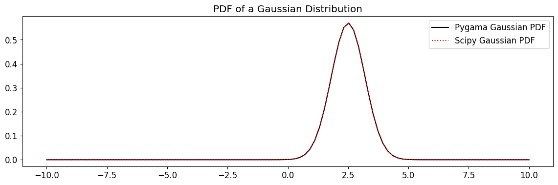
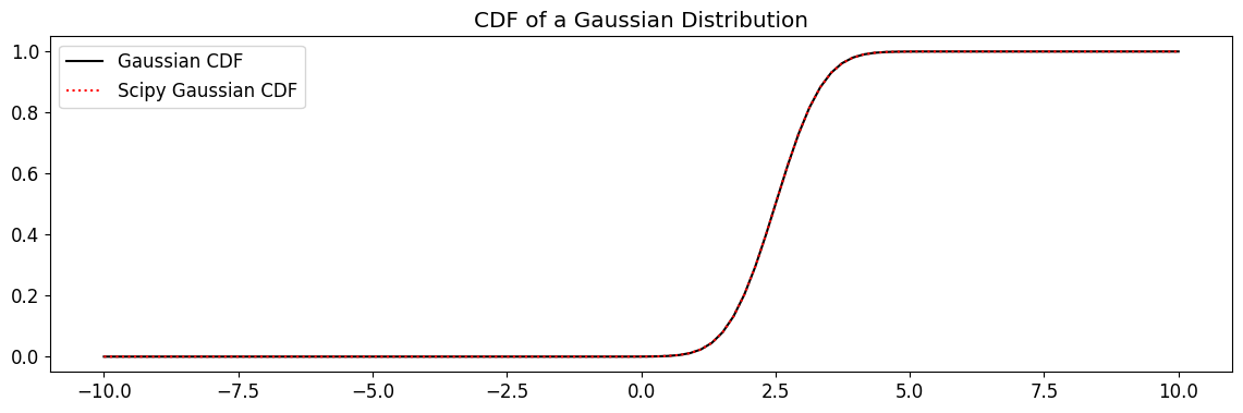
Geez, there are a lot of methods. Let’s hone in on a couple: ### .pdf and .cdf
These are just your bread and butter probability density and cumulative density functions
[3]:
gauss_pdf = gaussian.pdf(x, mu, sigma)

plt.plot(x, gauss_pdf, label="Pygama Gaussian PDF", c="k")
plt.plot(x, norm.pdf(x, mu, sigma), label="Scipy Gaussian PDF", ls=":", alpha=1, c="r")
plt.title("PDF of a Gaussian Distribution")
plt.legend()
plt.show()
[4]:
gauss_cdf = gaussian.cdf(x, mu, sigma)

plt.plot(x, gauss_cdf, label="Gaussian CDF", c="k")
plt.plot(x, norm.cdf(x, mu, sigma), label="Scipy Gaussian CDF", ls=":", alpha=1, c="r")
plt.title("CDF of a Gaussian Distribution")
plt.legend()
plt.show()
Ok, so that’s fine and dandy, what’s so special about a class that reproduces scipy results?
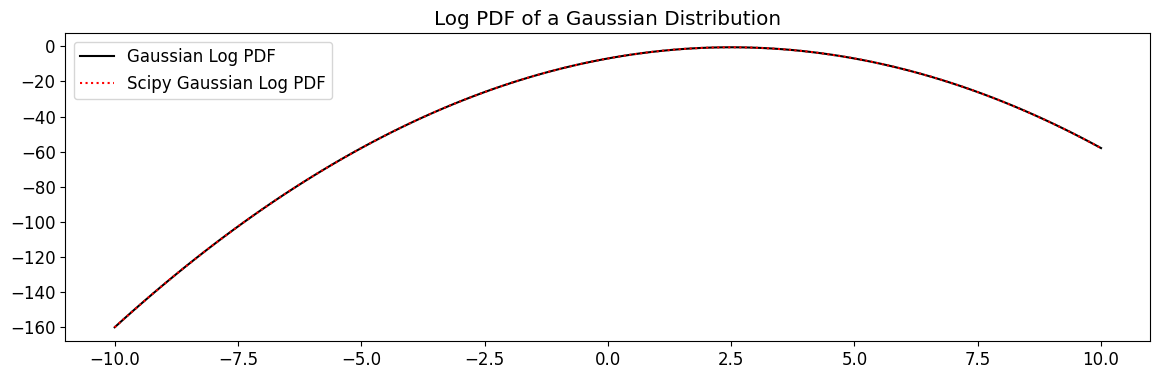
Well, every function in pygama.math.functions subclasses scipy’s rv_continuous class: this allows access to methods that scipy automagically computes. Let’s look at a few
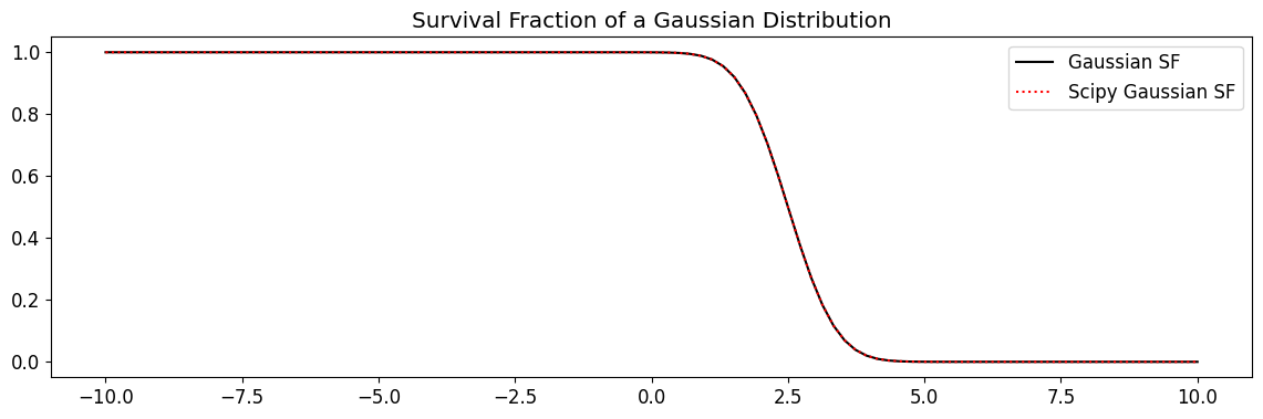
What rv_continuous subclassing gets us: .rvs, .logpdf, .sf…#
[5]:
gauss_log_pdf = gaussian.logpdf(x, mu, sigma)

plt.plot(x, gauss_log_pdf, label="Gaussian Log PDF", c="k")
plt.plot(
    x, norm.logpdf(x, mu, sigma), label="Scipy Gaussian Log PDF", ls=":", alpha=1, c="r"
)
plt.title("Log PDF of a Gaussian Distribution")
plt.legend()
plt.show()
[6]:
gauss_sf = gaussian.sf(x, mu, sigma)

plt.plot(x, gauss_sf, label="Gaussian SF", c="k")
plt.plot(x, norm.sf(x, mu, sigma), label="Scipy Gaussian SF", ls=":", alpha=1, c="r")
plt.title("Survival Fraction of a Gaussian Distribution")
plt.legend()
plt.show()
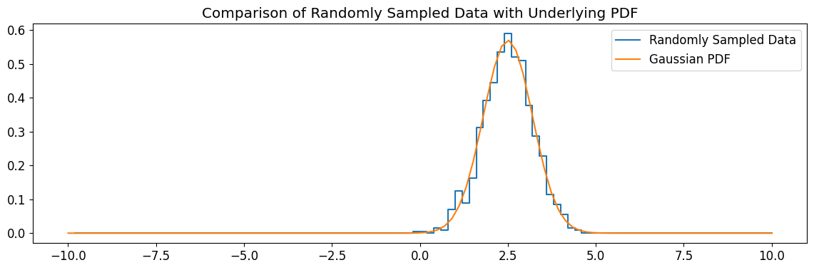
And now for something really useful, random sampling:
[7]:
random_sample = gaussian.rvs(mu, sigma, size=1000, random_state=1)

hist, bins = np.histogram(random_sample, bins=100, range=(-10, 10))
plt.step(
    bins[1:], hist / np.sum(hist) * np.sum(gauss_pdf), label="Randomly Sampled Data"
)
plt.plot(x, gauss_pdf, label="Gaussian PDF")
plt.title("Comparison of Randomly Sampled Data with Underlying PDF")
plt.legend()
plt.show()
We get access to scipy’s rv_continuous methods for free#
If we take a look at the actual code for the definition of pygama.math.functions.gaussian we see that there is no direct implementation of methods for .rvs or .logpdf! We get access to all these methods for free. All we have to do is subclass rv_continuous and write definitions for _pdf and _cdf
Now, the drawback: the functions _pdf and _cdf that rv_continuous uses are slow. Let’s see this by comparing to the function that actually computes the pdf: ### But the .pdf and .cdf methods are slow!
[8]:
%%timeit -r 4 -n 10000
gauss_pdf = gaussian.pdf(x, mu, sigma)
117 µs ± 281 ns per loop (mean ± std. dev. of 4 runs, 10,000 loops each)
[9]:
def gaussian_pdf(x, mu, sigma):
    if sigma == 0:
        invs = np.inf
    else:
        invs = 1.0 / sigma
    z = (x - mu) * invs
    invnorm = invs / np.sqrt(2 * np.pi)
    return np.exp(-0.5 * z**2) * invnorm
[10]:
%%timeit -r 4 -n 10000
gauss_pdf = gaussian_pdf(x, mu, sigma)
9 µs ± 122 ns per loop (mean ± std. dev. of 4 runs, 10,000 loops each)
Fast methods: .get_pdf and .get_cdf#
Because the overloaded rv_continuous implementations of pdf and cdf are very slow, we have implemented fast versions of these two methods, named get_pdf and get_cdf.
Each of these fast methods call a numba.njit-wrapped function — a just-in-time compiled function — that runs super fast.
We keep the .pdf and .cdf because they give us access to scipy methods we might want to use, but we write these faster methods so that we can fit distributions quickly.
[11]:
gauss_get_pdf = gaussian.get_pdf(x, mu, sigma)

plt.plot(x, gauss_get_pdf, label="Pygama Gaussian Get_PDF", c="k")
plt.plot(x, norm.pdf(x, mu, sigma), label="Scipy Gaussian PDF", ls=":", alpha=1, c="r")
plt.title("PDF of a Gaussian Distribution")
plt.legend()
plt.show()
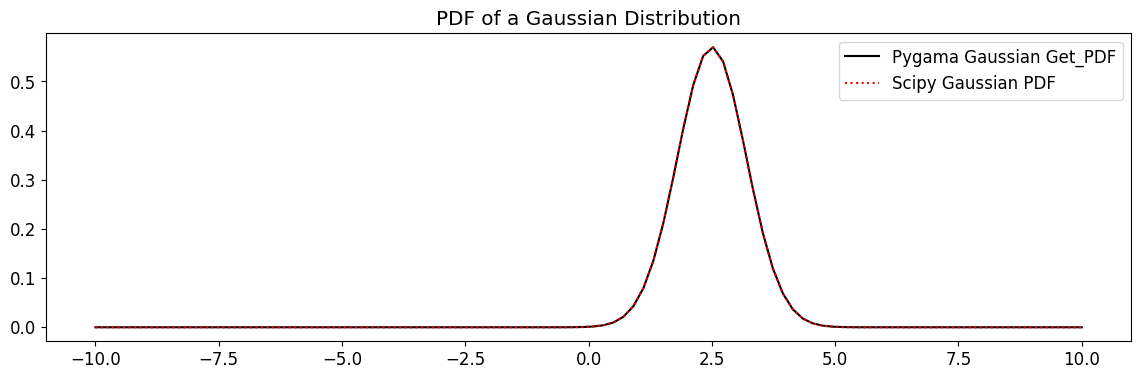
Ok, that’s good that it reproduces the scipy results numerically. But how fast does it run?
[12]:
%%timeit -r 4 -n 10000
gauss_pdf = gaussian.get_pdf(x, mu, sigma)
2.66 µs ± 50.2 ns per loop (mean ± std. dev. of 4 runs, 10,000 loops each)
See, we’re even faster than the function we defined above! That’s the power of just-in-time compiled code
The remaining methods are helpful for binned and unbinned fitting: norm_pdf, norm_cdf, pdf_ext and cdf_ext#
For pygama our default way of fitting distributions is to use the Iminuit package. Iminuit has several different ways to fit binned and unbinned data by performing either extended or unextended fits. These fitting methods require functions with different properties. The way pygama functions interact with Iminuit is as follows:
norm_pdfis used for unbinned fits, which require a pdf that is normalized to 1 on the fitting rangenorm_cdfis used for binned fits, which require a cdf that derived from a pdf that is normalized to 1 on the fitting rangepdf_extis used for extended unbinned fits, and the function is required to return a tuple of the support-normalized pdf integrated over the data window, and the scaled support-normalized pdf.cdf_extis used for extended binned fits, and just returns the scaled support-derived cdf
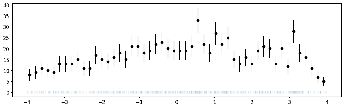
Let’s illustrate some fitting in action, and why some of these weird definitions are required ### Import Iminuit and create data to fit
[13]:
from iminuit import cost, Minuit

xr = (-4, 4)  # xrange
mu = 0.5
sigma = 3

rng = np.random.default_rng(1)

xdata = rng.normal(mu, sigma, size=1000)
xdata = xdata[(xr[0] < xdata) & (xdata < xr[1])]

n, xe = np.histogram(xdata, bins=50, range=xr)
cx = 0.5 * (xe[1:] + xe[:-1])
dx = np.diff(xe)

plt.errorbar(cx, n, n**0.5, fmt="ok")
plt.plot(xdata, np.zeros_like(xdata), "|", alpha=0.1);
Try an unbinned fit using the correct norm_pdf and the incorrect get_pdf#
We first note that the method norm_pdf has arguments x_lower, x_upper, mu, sigma where x_lower, x_upper are the bounds of the fitting range to ensure that the pdf is normalized to unity on. So, we therefore fix these fit parameters in Iminuit.
We also show a fit with get_pdf to show that the fit returns the incorrect results! We keep the get_pdf methods in pygama because they are useful if we ever need to numerically compute something quickly, or if we do a least squares fit.
[14]:
c = cost.UnbinnedNLL(xdata, gaussian.norm_pdf)

m_norm = Minuit(c, x_lower=xr[0], x_upper=xr[1], mu=0.4, sigma=0.2)
m_norm.fixed["x_lower", "x_upper"] = True
m_norm.limits["mu", "sigma"] = (0, None)
m_norm.migrad()
[14]:
| Migrad | ||||
|---|---|---|---|---|
| FCN = 3418 | Nfcn = 108 | |||
| EDM = 8.56e-07 (Goal: 0.0002) | time = 0.7 sec | |||
| Valid Minimum | No Parameters at limit | |||
| Below EDM threshold (goal x 10) | Below call limit | |||
| Covariance | Hesse ok | Accurate | Pos. def. | Not forced |
| Name | Value | Hesse Error | Minos Error- | Minos Error+ | Limit- | Limit+ | Fixed | |
|---|---|---|---|---|---|---|---|---|
| 0 | x_lower | -4.00 | 0.04 | yes | ||||
| 1 | x_upper | 4.00 | 0.04 | yes | ||||
| 2 | mu | 0.43 | 0.17 | 0 | ||||
| 3 | sigma | 3.10 | 0.24 | 0 |
| x_lower | x_upper | mu | sigma | |
|---|---|---|---|---|
| x_lower | 0 | 0 | 0 | 0 |
| x_upper | 0 | 0 | 0 | 0 |
| mu | 0 | 0 | 0.0287 | 0.0121 (0.300) |
| sigma | 0 | 0 | 0.0121 (0.300) | 0.0569 |
[15]:
c = cost.UnbinnedNLL(xdata, gaussian.get_pdf)

m = Minuit(c, mu=0.4, sigma=0.2)
m.limits["mu", "sigma"] = (0, None)
m.migrad()
[15]:
| Migrad | ||||
|---|---|---|---|---|
| FCN = 3570 | Nfcn = 90 | |||
| EDM = 3.38e-06 (Goal: 0.0002) | ||||
| Valid Minimum | No Parameters at limit | |||
| Below EDM threshold (goal x 10) | Below call limit | |||
| Covariance | Hesse ok | Accurate | Pos. def. | Not forced |
| Name | Value | Hesse Error | Minos Error- | Minos Error+ | Limit- | Limit+ | Fixed | |
|---|---|---|---|---|---|---|---|---|
| 0 | mu | 0.19 | 0.07 | 0 | ||||
| 1 | sigma | 2.06 | 0.05 | 0 |
| mu | sigma | |
|---|---|---|
| mu | 0.00508 | 2.25e-06 |
| sigma | 2.25e-06 | 0.00254 |
[16]:
plt.errorbar(cx, n, n**0.5, fmt="ok")
xm = np.linspace(*xr)
plt.plot(
    xm, gaussian.norm_pdf(xm, *m_norm.values) * len(xdata) * dx[0], label="norm_pdf fit"
)
plt.plot(xm, gaussian.get_pdf(xm, *m.values) * len(xdata) * dx[0], label="get_pdf fit")
plt.plot(
    xm, gaussian.get_pdf(xm, mu, sigma) * len(xdata) * dx[0], label="True Distribution"
)
plt.legend()
plt.show()
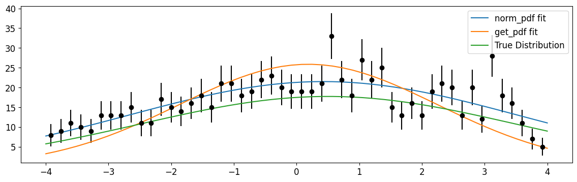
We see that norm_pdf does a much better job of fitting the actual underlying distribution and reproducing the correct \(\mu,\sigma\) parameters
try an extended unbinned fit#
The parameters for the pdf_ext are area, x_lo, x_hi, mu, sigma
[17]:
c = cost.ExtendedUnbinnedNLL(xdata, gaussian.pdf_ext)

m = Minuit(c, area=500, x_lo=xr[0], x_hi=xr[1], mu=0.1, sigma=0.9)
m.fixed["x_lo", "x_hi"] = True
m.limits["area", "mu", "sigma"] = (0, None)
m.migrad()
[17]:
| Migrad | ||||
|---|---|---|---|---|
| FCN = -6134 | Nfcn = 125 | |||
| EDM = 9.54e-06 (Goal: 0.0002) | time = 0.3 sec | |||
| Valid Minimum | No Parameters at limit | |||
| Below EDM threshold (goal x 10) | Below call limit | |||
| Covariance | Hesse ok | Accurate | Pos. def. | Not forced |
| Name | Value | Hesse Error | Minos Error- | Minos Error+ | Limit- | Limit+ | Fixed | |
|---|---|---|---|---|---|---|---|---|
| 0 | area | 1.04e3 | 0.06e3 | 0 | ||||
| 1 | x_lo | -4.00 | 0.04 | yes | ||||
| 2 | x_hi | 4.00 | 0.04 | yes | ||||
| 3 | mu | 0.43 | 0.17 | 0 | ||||
| 4 | sigma | 3.10 | 0.24 | 0 |
| area | x_lo | x_hi | mu | sigma | |
|---|---|---|---|---|---|
| area | 3.42e+03 | 0 | 0 | 3.02 (0.305) | 10.9 (0.783) |
| x_lo | 0 | 0 | 0 | 0 | 0 |
| x_hi | 0 | 0 | 0 | 0 | 0 |
| mu | 3.02 (0.305) | 0 | 0 | 0.0287 | 0.0122 (0.302) |
| sigma | 10.9 (0.783) | 0 | 0 | 0.0122 (0.302) | 0.0569 |
[18]:
plt.errorbar(cx, n, n**0.5, fmt="ok")
xm = np.linspace(*xr)
plt.plot(xm, gaussian.pdf_ext(xm, *m.values)[1] * dx[0], label="fit")
plt.plot(
    xm, gaussian.pdf_ext(xm, 1000, xr[0], xr[1], mu, sigma)[1] * dx[0], label="actual"
)
plt.legend()
plt.show()
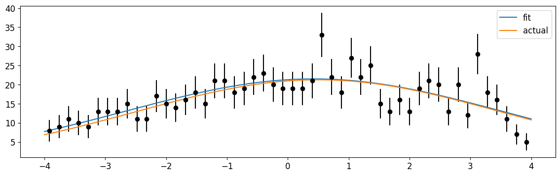
The pdf_ext function correctly fits the area of the curve!
Binned fits using norm_cdf and the incorrect get_cdf#
[19]:
c = cost.BinnedNLL(n, xe, gaussian.norm_cdf)

m_norm = Minuit(c, x_lower=xr[0], x_upper=xr[1], mu=0.4, sigma=0.2)
m_norm.fixed["x_lower", "x_upper"] = True
m_norm.limits["mu", "sigma"] = (0.1, None)
m_norm.migrad()
/home/docs/checkouts/readthedocs.org/user_builds/pygama/envs/refactor/lib/python3.10/site-packages/numpy/lib/function_base.py:1447: RuntimeWarning: invalid value encountered in subtract
  a = op(a[slice1], a[slice2])
[19]:
| Migrad | ||||
|---|---|---|---|---|
| FCN = 64.77 (chi2/ndof = 1.3) | Nfcn = 372 | |||
| EDM = 34.9 (Goal: 0.0002) | time = 0.6 sec | |||
| INVALID Minimum | No Parameters at limit | |||
| ABOVE EDM threshold (goal x 10) | Below call limit | |||
| Covariance | Hesse ok | Accurate | Pos. def. | Not forced |
| Name | Value | Hesse Error | Minos Error- | Minos Error+ | Limit- | Limit+ | Fixed | |
|---|---|---|---|---|---|---|---|---|
| 0 | x_lower | -4.00 | 0.04 | yes | ||||
| 1 | x_upper | 4.00 | 0.04 | yes | ||||
| 2 | mu | 1.4 | 1.7 | 0.1 | ||||
| 3 | sigma | 5.5 | 1.1 | 0.1 |
| x_lower | x_upper | mu | sigma | |
|---|---|---|---|---|
| x_lower | 0 | 0 | 0 | 0 |
| x_upper | 0 | 0 | 0 | 0 |
| mu | 0 | 0 | 3.83 | 2.21 (0.998) |
| sigma | 0 | 0 | 2.21 (0.998) | 1.28 |
[20]:
c = cost.BinnedNLL(n, xe, gaussian.get_cdf)

m = Minuit(c, mu=0.4, sigma=0.2)
m.limits["mu", "sigma"] = (0.1, None)
m.migrad()
[20]:
| Migrad | ||||
|---|---|---|---|---|
| FCN = 193.7 (chi2/ndof = 4.0) | Nfcn = 123 | |||
| EDM = 5.4e-07 (Goal: 0.0002) | ||||
| Valid Minimum | No Parameters at limit | |||
| Below EDM threshold (goal x 10) | Below call limit | |||
| Covariance | Hesse ok | Accurate | Pos. def. | Not forced |
| Name | Value | Hesse Error | Minos Error- | Minos Error+ | Limit- | Limit+ | Fixed | |
|---|---|---|---|---|---|---|---|---|
| 0 | mu | 0.19 | 0.07 | 0.1 | ||||
| 1 | sigma | 2.05 | 0.05 | 0.1 |
| mu | sigma | |
|---|---|---|
| mu | 0.00506 | -5.54e-07 |
| sigma | -5.54e-07 | 0.00253 |
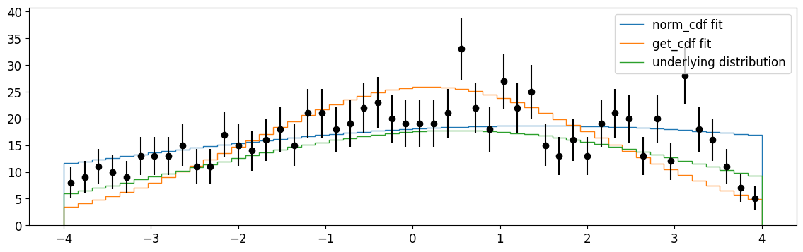
[21]:
plt.errorbar(cx, n, n**0.5, fmt="ok")
plt.stairs(
    np.diff(gaussian.norm_cdf(xe, *m_norm.values)) * len(xdata),
    xe,
    label="norm_cdf fit",
)
plt.stairs(
    np.diff(gaussian.get_cdf(xe, *m.values)) * len(xdata), xe, label="get_cdf fit"
)
plt.stairs(
    np.diff(gaussian.get_cdf(xe, mu, sigma)) * len(xdata),
    xe,
    label="underlying distribution",
)
plt.legend()
plt.show()
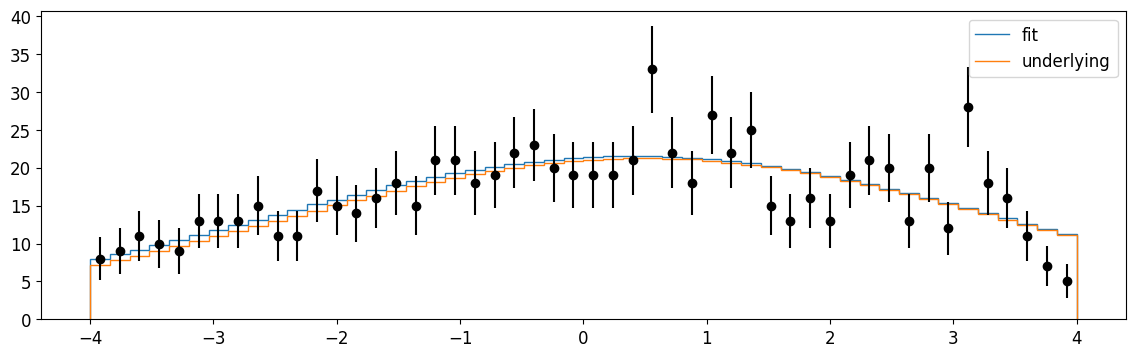
Finally, extended binned fits with cdf_ext#
[22]:
c = cost.ExtendedBinnedNLL(n, xe, gaussian.cdf_ext)

m = Minuit(c, area=500, mu=0.1, sigma=0.9)
m.limits["area", "mu", "sigma"] = (0, None)
m.migrad()
[22]:
| Migrad | ||||
|---|---|---|---|---|
| FCN = 42.85 (chi2/ndof = 0.9) | Nfcn = 128 | |||
| EDM = 4.11e-06 (Goal: 0.0002) | time = 0.5 sec | |||
| Valid Minimum | No Parameters at limit | |||
| Below EDM threshold (goal x 10) | Below call limit | |||
| Covariance | Hesse ok | Accurate | Pos. def. | Not forced |
| Name | Value | Hesse Error | Minos Error- | Minos Error+ | Limit- | Limit+ | Fixed | |
|---|---|---|---|---|---|---|---|---|
| 0 | area | 1.04e3 | 0.06e3 | 0 | ||||
| 1 | mu | 0.42 | 0.17 | 0 | ||||
| 2 | sigma | 3.08 | 0.23 | 0 |
| area | mu | sigma | |
|---|---|---|---|
| area | 3.3e+03 | 2.84 (0.297) | 10.4 (0.776) |
| mu | 2.84 (0.297) | 0.0279 | 0.0115 (0.295) |
| sigma | 10.4 (0.776) | 0.0115 (0.295) | 0.0547 |
[23]:
plt.errorbar(cx, n, n**0.5, fmt="ok")
plt.stairs(np.diff(gaussian.cdf_ext(xe, *m.values)), xe, label="fit")
plt.stairs(np.diff(gaussian.cdf_ext(xe, 1000, mu, sigma)), xe, label="underlying")
plt.legend();
Writing our own pygama.math distribution: conventions and requirements#
Let’s write a Cauchy distribution. Recall that a Cauchy distribution has support over the real line, and has a pdf like
\(pdf(x, \mu,\sigma) = \frac{1}{\pi\sigma\left[1+\left(\frac{x-\mu}{\sigma}\right)^2\right]}\)
and a cdf:
\(cdf(x, \mu,\sigma) = \frac{1}{\pi}\arctan\left(\frac{x-\mu}{\sigma}\right)+\frac{1}{2}\)
What we need to define a distribution class#
We need four functions that our class methods will call and their arguments, and they all should be numbafied
A PDF, normalized to the support. Args: x, mu, sigma
A CDF, derived from the support normalized PDF. Args: x, mu, sigma
A scaled PDF. Args: x, area, mu, sigma
A scaled CDF. Args: x, area, mu, sigma
The convention is to name these functions nb_distribution_pdf and nb_distribution_scaled_cdf for example.
[24]:
import numba as nb

# here we set some parameters to ensure that numba will compute things as quickly as possible
kwd_parallel = {"parallel": True, "fastmath": True}
kwd = {"parallel": False, "fastmath": True}

# define the pdf
@nb.njit(**kwd_parallel)
def nb_cauchy_pdf(x: np.ndarray, mu: float, sigma: float) -> np.ndarray:
    r"""
    Parameters
    ----------
    x
        The input data
    lamb
        The rate
    mu
        The amount to shift the distribution
    sigma
        The amount to scale the distribution
    """

    y = np.empty_like(x, dtype=np.float64)
    # we want to do a loop because it is faster with parallelization
    for i in nb.prange(x.shape[0]):
        y[i] = (x[i] - mu) / sigma
        y[i] = 1 / (np.pi * sigma * (1 + y[i] ** 2))
    return y


# define the cdf
@nb.njit(**kwd_parallel)
def nb_cauchy_cdf(x: np.ndarray, mu: float, sigma: float) -> np.ndarray:
    r"""
    Parameters
    ----------
    x
        The input data
    lamb
        The rate
    mu
        The amount to shift the distribution
    sigma
        The amount to scale the distribution
    """
    y = np.empty_like(x, dtype=np.float64)
    for i in nb.prange(x.shape[0]):
        y[i] = (x[i] - mu) / sigma
        y[i] = (1 / np.pi) * np.arctan(y[i]) + 0.5
    return y


# define the scaled pdf, can't use parallelization here because there is no outer for-loop
@nb.njit(**kwd)
def nb_cauchy_scaled_pdf(
    x: np.ndarray, area: float, mu: float, sigma: float
) -> np.ndarray:
    r"""
    Parameters
    ----------
    x
        The input data
    area
        The prefactor to scale the pdf by
    lamb
        The rate
    mu
        The amount to shift the distribution
    sigma
        The amount to scale the distribution
    """
    return area * nb_cauchy_pdf(x, mu, sigma)


# define the scaled cdf, can't use parallelization here because there is no outer for-loop
@nb.njit(**kwd)
def nb_cauchy_scaled_cdf(
    x: np.ndarray, area: float, mu: float, sigma: float
) -> np.ndarray:
    r"""
    Parameters
    ----------
    x
        The input data
    area
        The prefactor to scale the pdf by
    lamb
        The rate
    mu
        The amount to shift the distribution
    sigma
        The amount to scale the distribution
    """
    return area * nb_cauchy_cdf(x, mu, sigma)
Now we create a class using these four functions#
Each pygama distribution class subclasses pygama_continuous, which itself is a subclass of rv_continuous.
An aside on the ordering of parameters:#
In the following the term “shape parameter” refers to a specific variable used to define a distribution that is not an overall scaling (which I call \(\mu\)) or shifting (which I call \(\sigma\)). An example of shape parameters would be the \(\beta, m\) parameters in a crystal ball function. The location and scale (\(\mu, \sigma\)) parameters have a more specific definition — akin to what scipy does. If a \(\mu, \sigma\) value is present, then the entire distribution is
shifted and scaled; this can be achieved by transforming \(y = \frac{x-\mu}{\sigma}\) and computing \(pdf(y)/\sigma\) ( where the factor of \(1/\sigma\) comes from the Jacobian).
The ordering of parameters is as follows, using whichever are needed for a function: x, area, x_lower, x_upper, shapes, ..., mu, sigma
Where x_lower and x_upper are the lower and upper bounds to evaluate a function on.
Now, back to require methods#
The class name has the format distribution_name_gen and it must include the following methods with their arguments:
_pdf(self, x, shapes):This is an overloading of the
scipymethod for the pdf. Becausescipyfirst computes \(\frac{x-\mu}{\sigma}\) and \(pdf/\sigma\), we need to callnb_distribution_pdfwith \(\mu = 0\) and \(\sigma = 1\). If shape parameters are present,nb_distribution_pdfmust also be called withshape_param[0]becausescipypasses an array of shape parameters to the function calls. Finally,x.flags.writeable = Truemust be passed so thatnumbacan operate as expected on arrays._cdf(self, x, shapes):This is an overloading of the
scipymethod for the cdf. The same format applies as for the pdf.get_pdf(x, shapes, mu, sigma):This is a direct call to the fast
nb_distribution_pdfget_pdf(x, shapes, mu, sigma):This is a direct call to the fast
nb_distribution_cdfnorm_pdf(x, x_lower, x_upper, shapes, mu, sigma):In the case that the support of the distribution is the entire real line, this calls a
pygama_continuoussuper method that normalizes the pdf to unity on the range \([x_{lower},x_{upper}]\) by computing \(\frac{pdf(x)}{cdf(x_{upper})- cdf(x_{lower})}\). If the distribution is defined on a limited domain, this function needs to be directly overloaded – seepygama.math.functions.stepfor an example.norm_cdf(x, x_lower, x_upper, shapes, mu, sigma):In the case that the support of the distribution is the entire real line, this calls a
pygama_continuoussuper method that derives the cdf from a pdf that is normalized to unity on the range \([x_{lower},x_{upper}]\) by computing \(\frac{cdf(x)}{cdf(x_{upper})- cdf(x_{lower})}\). If the distribution is defined on a limited domain, this function needs to be directly overloaded – seepygama.math.functions.stepfor an example.pdf_ext(x, area, x_lower, x_upper, shapes, mu, sigma):A function that returns both the integral of the support-normalized pdf on the interval \([x_{lower},x_{upper}]\), as well as the support-normalized pdf on that range as well. The fastest way to compute these is to return
np.diff(nb_distribution_scaled_cdf(np.array([x_lower, x_upper]), area, shapes, mu, sigma))andnb_distribution_scaled_pdf(x, area, shapes, mu, sigma)cdf_ext(x, area, shapes, mu, sigma):A function that returns just the scaled cdf,
nb_distribution_scaled_cdf(x, area, shapes, mu, sigma)req_args(self):A function that returns a tuple with the strings of the names of the required shape parameters and mu and sigma
[25]:
from pygama.math.functions.pygama_continuous import pygama_continuous


class cauchy_gen(pygama_continuous):
    def _pdf(self, x: np.ndarray) -> np.ndarray:
        x.flags.writeable = True
        return nb_cauchy_pdf(x, 0, 1)

    def _cdf(self, x: np.ndarray) -> np.ndarray:
        x.flags.writeable = True
        return nb_cauchy_cdf(x, 0, 1)

    def get_pdf(self, x: np.ndarray, mu: float, sigma: float) -> np.ndarray:
        return nb_cauchy_pdf(x, mu, sigma)

    def get_cdf(self, x: np.ndarray, mu: float, sigma: float) -> np.ndarray:
        return nb_cauchy_cdf(x, mu, sigma)

    # needed so that we can hack iminuit's introspection to function parameter names.
    def norm_pdf(
        self, x: np.ndarray, x_lower: float, x_upper: float, mu: float, sigma: float
    ) -> np.ndarray:
        return self._norm_pdf(x, x_lower, x_upper, mu, sigma)

    def norm_cdf(
        self, x: np.ndarray, x_lower: float, x_upper: float, mu: float, sigma: float
    ) -> np.ndarray:
        return self._norm_cdf(x, x_lower, x_upper, mu, sigma)

    def pdf_ext(
        self,
        x: np.ndarray,
        area: float,
        x_lower: float,
        x_upper: float,
        mu: float,
        sigma: float,
    ) -> np.ndarray:
        return np.diff(
            nb_cauchy_scaled_cdf(np.array([x_lower, x_upper]), area, mu, sigma)
        ), nb_cauchy_scaled_pdf(x, area, mu, sigma)

    def cdf_ext(
        self, x: np.ndarray, area: float, mu: float, sigma: float
    ) -> np.ndarray:
        return nb_cauchy_scaled_cdf(x, area, mu, sigma)

    def required_args(self) -> tuple[str, str]:
        return "mu", "sigma"


cauchy = cauchy_gen(name="cauchy")
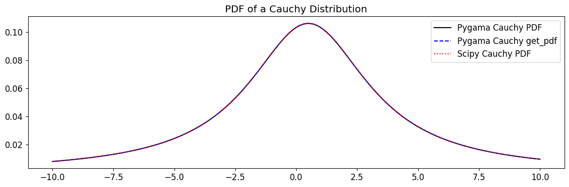
[26]:
from scipy.stats import cauchy as scipy_cauchy
cauchy_pdf = cauchy.pdf(x, mu, sigma)
cauchy_get_pdf = cauchy.get_pdf(x, mu, sigma)
cauchy_cdf = cauchy.cdf(x, mu, sigma)
cauchy_get_cdf = cauchy.get_cdf(x, mu, sigma)
plt.plot(x, cauchy_pdf, label="Pygama Cauchy PDF", c="k")
plt.plot(x, cauchy_get_pdf, label="Pygama Cauchy get_pdf", c="b", ls="--")
plt.plot(
x, scipy_cauchy.pdf(x, mu, sigma), label="Scipy Cauchy PDF", ls=":", alpha=1, c="r"
)
plt.title("PDF of a Cauchy Distribution")
plt.legend()
plt.show()
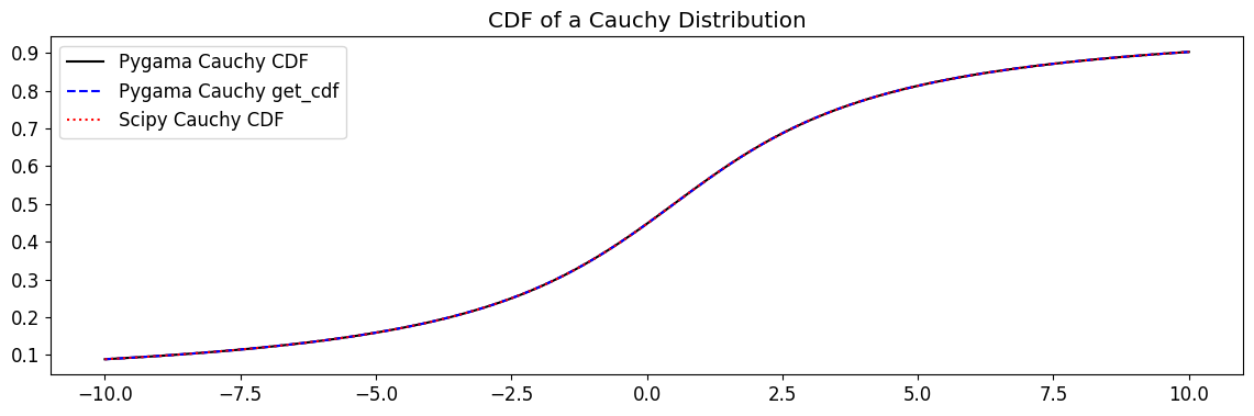
plt.plot(x, cauchy_cdf, label="Pygama Cauchy CDF", c="k")
plt.plot(x, cauchy_get_cdf, label="Pygama Cauchy get_cdf", c="b", ls="--")
plt.plot(
x, scipy_cauchy.cdf(x, mu, sigma), label="Scipy Cauchy CDF", ls=":", alpha=1, c="r"
)
plt.title("CDF of a Cauchy Distribution")
plt.legend()
plt.show()
Perform some fits using the new Cauchy distribution to show the other methods’ validity#
[27]:
xr = (-4, 4) # xrange
mu = 0.5
sigma = 0.7
xdata = scipy_cauchy.rvs(mu, sigma, size=1000, random_state=42)
xdata = xdata[(xr[0] < xdata) & (xdata < xr[1])]
n, xe = np.histogram(xdata, bins=50, range=xr)
cx = 0.5 * (xe[1:] + xe[:-1])
dx = np.diff(xe)
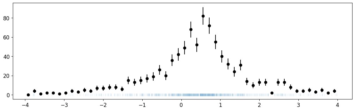
plt.errorbar(cx, n, n**0.5, fmt="ok")
plt.plot(xdata, np.zeros_like(xdata), "|", alpha=0.1);
unbinned fit#
[28]:
c = cost.UnbinnedNLL(xdata, cauchy.norm_pdf)

m_norm = Minuit(c, x_lower=xr[0], x_upper=xr[1], mu=0.4, sigma=0.2)
m_norm.fixed["x_lower", "x_upper"] = True
m_norm.limits["mu", "sigma"] = (0, None)
m_norm.migrad()
[28]:
| Migrad | ||||
|---|---|---|---|---|
| FCN = 2784 | Nfcn = 56 | |||
| EDM = 1.66e-07 (Goal: 0.0002) | time = 0.7 sec | |||
| Valid Minimum | No Parameters at limit | |||
| Below EDM threshold (goal x 10) | Below call limit | |||
| Covariance | Hesse ok | Accurate | Pos. def. | Not forced |
| Name | Value | Hesse Error | Minos Error- | Minos Error+ | Limit- | Limit+ | Fixed | |
|---|---|---|---|---|---|---|---|---|
| 0 | x_lower | -4.00 | 0.04 | yes | ||||
| 1 | x_upper | 4.00 | 0.04 | yes | ||||
| 2 | mu | 0.478 | 0.033 | 0 | ||||
| 3 | sigma | 0.73 | 0.04 | 0 |
| x_lower | x_upper | mu | sigma | |
|---|---|---|---|---|
| x_lower | 0 | 0 | 0 | 0 |
| x_upper | 0 | 0 | 0 | 0 |
| mu | 0 | 0 | 0.00106 | -2.25e-05 (-0.018) |
| sigma | 0 | 0 | -2.25e-05 (-0.018) | 0.00147 |
extended unbinned fit#
[29]:
c = cost.ExtendedUnbinnedNLL(xdata, cauchy.pdf_ext)

m = Minuit(c, area=500, x_lower=xr[0], x_upper=xr[1], mu=0.1, sigma=0.9)
m.fixed["x_lower", "x_upper"] = True
m.limits["area", "mu", "sigma"] = (0.01, None)
m.migrad()
[29]:
| Migrad | ||||
|---|---|---|---|---|
| FCN = -7457 | Nfcn = 102 | |||
| EDM = 2.22e-07 (Goal: 0.0002) | time = 0.3 sec | |||
| Valid Minimum | No Parameters at limit | |||
| Below EDM threshold (goal x 10) | Below call limit | |||
| Covariance | Hesse ok | Accurate | Pos. def. | Not forced |
| Name | Value | Hesse Error | Minos Error- | Minos Error+ | Limit- | Limit+ | Fixed | |
|---|---|---|---|---|---|---|---|---|
| 0 | area | 1.002e3 | 0.034e3 | 0.01 | ||||
| 1 | x_lower | -4.00 | 0.04 | yes | ||||
| 2 | x_upper | 4.00 | 0.04 | yes | ||||
| 3 | mu | 0.478 | 0.033 | 0.01 | ||||
| 4 | sigma | 0.73 | 0.04 | 0.01 |
| area | x_lower | x_upper | mu | sigma | |
|---|---|---|---|---|---|
| area | 1.18e+03 | 0 | 0 | 0.00417 | 0.26 (0.197) |
| x_lower | 0 | 0 | 0 | 0 | 0 |
| x_upper | 0 | 0 | 0 | 0 | 0 |
| mu | 0.00417 | 0 | 0 | 0.00106 | -2.19e-05 (-0.018) |
| sigma | 0.26 (0.197) | 0 | 0 | -2.19e-05 (-0.018) | 0.00147 |
Binned fit#
[30]:
c = cost.BinnedNLL(n, xe, cauchy.norm_cdf)

m_norm = Minuit(c, x_lower=xr[0], x_upper=xr[1], mu=0.4, sigma=0.2)
m_norm.fixed["x_lower", "x_upper"] = True
m_norm.limits["mu", "sigma"] = (0.1, None)
m_norm.migrad()
[30]:
| Migrad | ||||
|---|---|---|---|---|
| FCN = 52.27 (chi2/ndof = 1.1) | Nfcn = 48 | |||
| EDM = 3.04e-05 (Goal: 0.0002) | ||||
| Valid Minimum | No Parameters at limit | |||
| Below EDM threshold (goal x 10) | Below call limit | |||
| Covariance | Hesse ok | Accurate | Pos. def. | Not forced |
| Name | Value | Hesse Error | Minos Error- | Minos Error+ | Limit- | Limit+ | Fixed | |
|---|---|---|---|---|---|---|---|---|
| 0 | x_lower | -4.00 | 0.04 | yes | ||||
| 1 | x_upper | 4.00 | 0.04 | yes | ||||
| 2 | mu | 0.482 | 0.033 | 0.1 | ||||
| 3 | sigma | 0.73 | 0.04 | 0.1 |
| x_lower | x_upper | mu | sigma | |
|---|---|---|---|---|
| x_lower | 0 | 0 | 0 | 0 |
| x_upper | 0 | 0 | 0 | 0 |
| mu | 0 | 0 | 0.00107 | -2.99e-05 (-0.024) |
| sigma | 0 | 0 | -2.99e-05 (-0.024) | 0.00149 |
Extended binned fit#
[31]:
c = cost.ExtendedBinnedNLL(n, xe, cauchy.cdf_ext)

m = Minuit(c, area=500, mu=0.1, sigma=0.9)
m.limits["area", "mu", "sigma"] = (0, None)
m.migrad()
[31]:
| Migrad | ||||
|---|---|---|---|---|
| FCN = 52.27 (chi2/ndof = 1.1) | Nfcn = 95 | |||
| EDM = 6.18e-06 (Goal: 0.0002) | ||||
| Valid Minimum | No Parameters at limit | |||
| Below EDM threshold (goal x 10) | Below call limit | |||
| Covariance | Hesse ok | Accurate | Pos. def. | Not forced |
| Name | Value | Hesse Error | Minos Error- | Minos Error+ | Limit- | Limit+ | Fixed | |
|---|---|---|---|---|---|---|---|---|
| 0 | area | 1.002e3 | 0.034e3 | 0 | ||||
| 1 | mu | 0.483 | 0.033 | 0 | ||||
| 2 | sigma | 0.73 | 0.04 | 0 |
| area | mu | sigma | |
|---|---|---|---|
| area | 1.18e+03 | 0.00298 | 0.264 (0.199) |
| mu | 0.00298 | 0.00107 | -2.98e-05 (-0.024) |
| sigma | 0.264 (0.199) | -2.98e-05 (-0.024) | 0.00149 |
Adding distributions with sum_dists#
In the business of fitting data, adding two distributions together is our bread-and-butter. This part of the notebook will show you how to create your own distribution that subclasses pygama.math.sum_dists. There are a couple of different use cases for adding distributions together, and we will look at each in turn, but here is a summary:
Adding different fractions of distributions together, and fitting out the relative amount of distributions
Adding distributions with different areas (present in equal fractions) and fitting the areas
Adding distributions with different areas that have different fractions, and fitting out the areas and fractions
Let’s first create the synthetic data that we will fit#
[32]:
xr = (-4, 4) # xrange
rng = np.random.default_rng(1)
mu = 0.5
sigma = 1.3
mu2 = 1
sigma2 = 0.6
xdata = norm.rvs(mu, sigma, size=1000, random_state=42)
ydata = scipy_cauchy.rvs(mu2, sigma2, size=len(xdata), random_state=42)
xmix = np.append(xdata, ydata)
xmix = xmix[(xr[0] < xmix) & (xmix < xr[1])]
n, xe = np.histogram(xmix, bins=50, range=xr)
cx = 0.5 * (xe[1:] + xe[:-1])
dx = np.diff(xe)
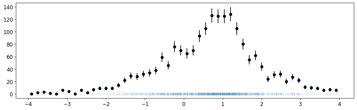
plt.errorbar(cx, n, n**0.5, fmt="ok")
plt.plot(xmix, np.zeros_like(xmix), "|", alpha=0.1);
A little about sum_dists#
The first important thing to note about this class is that all method class are of the form method(x, parameter_array). We want to use a single array as an argument because we need to accommodate an arbitrarily large number of parameters. In addition, a single array is an acceptable input for Iminuit fits.
So, the first thing a user does in creating a new class is define the order of elements in a parameter_array. Now, sum_dists works by grabbing elements at different indices in this parameter_array according to rules that the user provides in the __init__. Here’s how to write a generic class:
Create a
parameter_index_arraythat holds the indices of what will eventually come in theparameter_array. If the user will eventually passparameters = [frac1, mu, sigma]then we just takeparameter_index_array=[frac1, mu, sigma]=range(3)sum_diststakes an alternating pattern of distributions and distribution-specific parameter_index_arrays. Each par array can contain[shape, mu, sigma, area, frac]with area and frac being optional (depending on the flag sent to the constructor) but must be placed in that order.We pass one of the 4 flag options, to be described below.
Let’s trace through how the code works for a simple example. Suppose we want to create the following distribution
\(new\_pdf(x, [\tau, \mu, \sigma, frac_1, frac_2]) = frac_1\cdot dist_1(x, \tau, \mu, \sigma) + frac_2\cdot dist_2(x, \mu, \sigma)\)
The first thing we would do is create our parameter_index_array
[tau, mu, sigma, frac_1, frac_2] = range(5)
Then, we would create our alternating pattern of distributions and parameter index arrays:
args = [dist1, [tau, mu, sigma, frac_1], dist2, [mu, sigma, frac2]]
Finally, we would intitalize (with the fracs flag in this case, more on that later)
super().__init__(*args, frac_flag = "fracs")
So… What is sum_dists actually doing?#
Under the hood, sum_dists is applying a set of rules so that the following is always computed, regardless of the flag sent to the constructor.
total_area*area1*frac1*dist1(x, shape, mu, sigma) + ... total_area*area_n*frac_n*dist_n(x, shape_1, mu_n, sigma_n)
It does this by first reading through all of the parameter index arrays for each distribution and separating the indices for the shape parameters, areas, and fracs into separate index arrays. Then, at the time of method call, these separate parameter index arrays are used to grab the actual values for the shape parameters, fractions, and areas. There’s also some work done to determine which of area and frac are present. That’s the purpose of the frac_flag. Let’s take some time and
learn a little more about what each flag does.
The areas flag in the sum_dists constructor#
Let’s say we are interested in knowing the amount of counts present in a signal and a background in our total spectrum, i.e. we want to create and fit a function that looks like
\(pdf= A\cdot gauss\_pdf + B\cdot cauchy\_pdf\)
Because we are interested in fitting the areas, we send the areas keyword to frac_flag. This causes sum_dists to assume that the last element in each parameter index array in the constructor is an area for that specific distribution. By default, all the fracs are set to 1, as well as the total_area.
[33]:
from pygama.math.functions.sum_dists import sum_dists


class cauchy_on_gauss_gen(sum_dists):
    def __init__(self):
        # we first create an array contains the indices of the parameter array
        # that will eventually be input to function calls
        (area1, mu, sigma, area2, mu2, sigma2) = range(6)

        # we now create an array containing the distributions and their shape parameters
        # The last item in a parameter array is the fraction or area component
        # The last item in the last parameter array corresponds to the total area, if present
        # but because we are fitting individual areas, the total area is meaningless
        args = [gaussian, [mu, sigma, area1], cauchy, [mu2, sigma2, area2]]
        # we initialize with the frac_flag = "areas" to let the constructor know we are sending frac parameters only
        super().__init__(*args, frac_flag="areas")

    def get_req_args(self) -> tuple[str, str, str]:
        r"""
        Return the required arguments for this instance
        """
        return "area1", "mu", "sigma", "area2", "mu2", "sigma2"


cauchy_on_gauss = cauchy_on_gauss_gen()
That was super quick, let’s see how it does with fitting data#
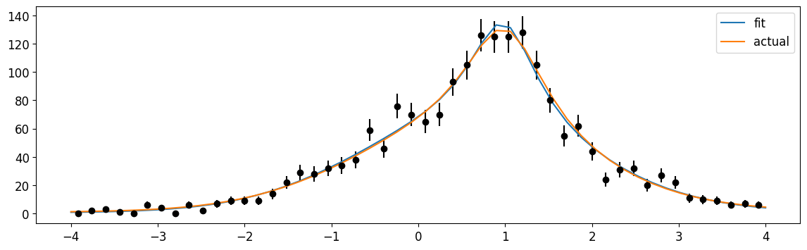
Because we are interested in fitting out areas, we need to use the extended forms of our fits And for pdf_ext methods we have two options: we either pass x_lo, x_hi at the start of our parameter array, or we don’t pass them and the function automatically takes the np.amin(x), np.amax(x) as those values
something to note: all parameter arrays passed to sum_dist methods must be numpy arrays; for example, see that we must turn m.values into np.array(m.values) in order for it to work#
[34]:
c = cost.ExtendedUnbinnedNLL(xmix, cauchy_on_gauss.pdf_ext)

m = Minuit(c, (xr[0], xr[1], 100, 0.1, 0.3, 100, 1, 2))
m.fixed[0, 1] = True  # fix the x_lo, x_hi
m.limits[2, 5] = (0, None)
m.limits[3, 4, 6, 7] = (0, 2)
print(m.migrad())

plt.errorbar(cx, n, n**0.5, fmt="ok")
xm = np.linspace(*xr)
plt.plot(xm, cauchy_on_gauss.pdf_ext(xm, np.array(m.values))[1] * dx[0], label="fit")
plt.plot(
    xm,
    cauchy_on_gauss.pdf_ext(xm, np.array([1000, mu, sigma, 1000, mu2, sigma2]))[1]
    * dx[0],
    label="actual",
)
plt.legend();
┌─────────────────────────────────────────────────────────────────────────┐
│                                Migrad                                   │
├──────────────────────────────────┬──────────────────────────────────────┤
│ FCN = -1.875e+04                 │              Nfcn = 408              │
│ EDM = 9.35e-05 (Goal: 0.0002)    │            time = 0.9 sec            │
├──────────────────────────────────┼──────────────────────────────────────┤
│          Valid Minimum           │        No Parameters at limit        │
├──────────────────────────────────┼──────────────────────────────────────┤
│ Below EDM threshold (goal x 10)  │           Below call limit           │
├───────────────┬──────────────────┼───────────┬─────────────┬────────────┤
│  Covariance   │     Hesse ok     │ Accurate  │  Pos. def.  │ Not forced │
└───────────────┴──────────────────┴───────────┴─────────────┴────────────┘
┌───┬──────┬───────────┬───────────┬────────────┬────────────┬─────────┬─────────┬───────┐
│   │ Name │   Value   │ Hesse Err │ Minos Err- │ Minos Err+ │ Limit-  │ Limit+  │ Fixed │
├───┼──────┼───────────┼───────────┼────────────┼────────────┼─────────┼─────────┼───────┤
│ 0 │ x0   │   -4.00   │   0.04    │            │            │         │         │  yes  │
│ 1 │ x1   │   4.00    │   0.04    │            │            │         │         │  yes  │
│ 2 │ x2   │  1.19e3   │  0.15e3   │            │            │    0    │         │       │
│ 3 │ x3   │   0.57    │   0.07    │            │            │    0    │    2    │       │
│ 4 │ x4   │   1.32    │   0.05    │            │            │    0    │    2    │       │
│ 5 │ x5   │  0.78e3   │  0.17e3   │            │            │    0    │         │       │
│ 6 │ x6   │   0.98    │   0.04    │            │            │    0    │    2    │       │
│ 7 │ x7   │   0.50    │   0.09    │            │            │    0    │    2    │       │
└───┴──────┴───────────┴───────────┴────────────┴────────────┴─────────┴─────────┴───────┘
┌────┬─────────────────────────────────────────────────────────────────────────────────┐
│    │        x0        x1        x2        x3        x4        x5        x6        x7 │
├────┼─────────────────────────────────────────────────────────────────────────────────┤
│ x0 │         0         0         0         0         0         0         0         0 │
│ x1 │         0         0         0         0         0         0         0         0 │
│ x2 │         0         0  2.17e+04      6.02      2.27 -2.38e+04     0.492     -10.9 │
│ x3 │         0         0      6.02   0.00465  0.000935     -6.86 -0.000945  -0.00302 │
│ x4 │         0         0      2.27  0.000935   0.00242      -2.7 -0.000432   -0.0023 │
│ x5 │         0         0 -2.38e+04     -6.86      -2.7  2.84e+04    -0.587      12.8 │
│ x6 │         0         0     0.492 -0.000945 -0.000432    -0.587   0.00194 -0.000165 │
│ x7 │         0         0     -10.9  -0.00302   -0.0023      12.8 -0.000165   0.00805 │
└────┴─────────────────────────────────────────────────────────────────────────────────┘
Well, that’s pretty good! Let’s see how the extended unbinned fit fairs
[35]:
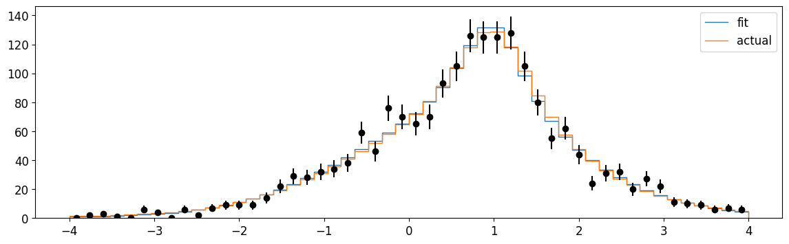
c = cost.ExtendedBinnedNLL(n, xe, cauchy_on_gauss.cdf_ext)
m = Minuit(c, (100, 0.1, 0.3, 100, 1, 2))
m.limits[0, 3] = (0, None)
m.limits[1, 2, 4, 5] = (0, 2)
print(m.migrad())

plt.errorbar(cx, n, n**0.5, fmt="ok")
plt.stairs(np.diff(cauchy_on_gauss.cdf_ext(xe, np.array(m.values))), xe, label="fit")
plt.stairs(
    np.diff(
        cauchy_on_gauss.cdf_ext(xe, np.array([1000, mu, sigma, 1000, mu2, sigma2]))
    ),
    xe,
    label="actual",
)
plt.legend();
┌─────────────────────────────────────────────────────────────────────────┐
│                                Migrad                                   │
├──────────────────────────────────┬──────────────────────────────────────┤
│ FCN = 58.66 (chi2/ndof = 1.3)    │              Nfcn = 461              │
│ EDM = 9.22e-05 (Goal: 0.0002)    │                                      │
├──────────────────────────────────┼──────────────────────────────────────┤
│          Valid Minimum           │        No Parameters at limit        │
├──────────────────────────────────┼──────────────────────────────────────┤
│ Below EDM threshold (goal x 10)  │           Below call limit           │
├───────────────┬──────────────────┼───────────┬─────────────┬────────────┤
│  Covariance   │     Hesse ok     │ Accurate  │  Pos. def.  │ Not forced │
└───────────────┴──────────────────┴───────────┴─────────────┴────────────┘
┌───┬──────┬───────────┬───────────┬────────────┬────────────┬─────────┬─────────┬───────┐
│   │ Name │   Value   │ Hesse Err │ Minos Err- │ Minos Err+ │ Limit-  │ Limit+  │ Fixed │
├───┼──────┼───────────┼───────────┼────────────┼────────────┼─────────┼─────────┼───────┤
│ 0 │ x0   │  1.20e3   │  0.14e3   │            │            │    0    │         │       │
│ 1 │ x1   │   0.57    │   0.06    │            │            │    0    │    2    │       │
│ 2 │ x2   │   1.32    │   0.05    │            │            │    0    │    2    │       │
│ 3 │ x3   │  0.77e3   │  0.15e3   │            │            │    0    │         │       │
│ 4 │ x4   │   0.98    │   0.05    │            │            │    0    │    2    │       │
│ 5 │ x5   │   0.49    │   0.08    │            │            │    0    │    2    │       │
└───┴──────┴───────────┴───────────┴────────────┴────────────┴─────────┴─────────┴───────┘
┌────┬─────────────────────────────────────────────────────────────┐
│    │        x0        x1        x2        x3        x4        x5 │
├────┼─────────────────────────────────────────────────────────────┤
│ x0 │  1.82e+04      4.66      1.48 -1.96e+04     0.631     -9.06 │
│ x1 │      4.66   0.00388  0.000735     -5.31 -0.000857  -0.00235 │
│ x2 │      1.48  0.000735   0.00208     -1.76 -0.000397  -0.00177 │
│ x3 │ -1.96e+04     -5.31     -1.76  2.35e+04    -0.736      10.7 │
│ x4 │     0.631 -0.000857 -0.000397    -0.736   0.00203 -0.000313 │
│ x5 │     -9.06  -0.00235  -0.00177      10.7 -0.000313   0.00708 │
└────┴─────────────────────────────────────────────────────────────┘
The fracs flag in the sum_dists constructor#
To get a feel for how sum_dists works, let’s create a function that creates the following distribution:
\(pdf = f_1\cdot gauss\_{pdf}+(1-f_1)\cdot cauchy\_{pdf}\)
Well, it might seem crazy, but we can actually link together parameters before they are fit! That’s the beauty of the parameter index array and the link_pars function that we can overload.
The fracs keyword causes sum_dists to assume the following about the parameter index arrays in the __init__: each parameter index array looks like [shapes, mu, sigma, frac] with the exception of the last parameter index array which has the form [shapes, mu, sigma, frac, total_area].
Well, what if we don’t care about total_area? Or, what if we want to link parameters, like the f_1 value in the above example? That’s where link_pars comes in. Nominally, link_pars serves to extract the actual values of the shapes, fracs, and areas from the passed parameter array. But, if we overload it, we can actually link the parameters together! See the below code for an example.
[36]:
from pygama.math.functions.sum_dists import sum_dists


class cauchy_on_gauss_gen(sum_dists):
    def __init__(self):
        # we first create an array contains the indices of the parameter array
        # that will eventually be input to function calls
        (frac1, mu, sigma, mu2, sigma2) = range(5)

        # we now create an array containing the distributions and their shape parameters
        # The last item in a parameter array is the fraction or area component
        # The last item in the last parameter array corresponds to the total area if present
        args = [gaussian, [mu, sigma, frac1], cauchy, [mu2, sigma2, frac1, frac1]]
        # we initialize with the frac_flag = "fracs" to let the constructor know we are sending frac parameters only
        super().__init__(*args, frac_flag="fracs")

    def _link_pars(
        self,
        shape_par_idx,
        area_idx,
        frac_idx,
        total_area_idx,
        params,
        areas,
        fracs,
        total_area,
    ):
        shape_pars, cum_len, areas, fracs, total_area = super()._link_pars(
            shape_par_idx,
            area_idx,
            frac_idx,
            total_area_idx,
            params,
            areas,
            fracs,
            total_area,
        )

        fracs[1] = (
            1 - fracs[0]
        )  # create :math:`(1-frac1)` for the cauchy, and :math:`frac1` for the exgauss
        total_area[
            0
        ] = 1  # just overwrite the total area because we don't want to fit it

        return shape_pars, cum_len, areas, fracs, total_area

    def get_req_args(self) -> tuple[str, str, str]:
        r"""
        Return the required arguments for this instance
        """
        return "frac1", "mu", "sigma", "mu2", "sigma2"


cauchy_on_gauss = cauchy_on_gauss_gen()
Again, that was painless; let’s see how well it does fitting data#
[37]:
c = cost.UnbinnedNLL(xmix, cauchy_on_gauss.norm_pdf)

m = Minuit(c, (xr[0], xr[1], 0.5, 0.1, 0.2, 1, 0.1))
m.fixed[0, 1] = True
m.limits[2] = (0, 1)
m.limits[3, 4, 5, 6] = (0.5, 2)
print(m.migrad())

plt.errorbar(cx, n, n**0.5, fmt="ok")
xm = np.linspace(*xr)
plt.plot(
    xm,
    cauchy_on_gauss.norm_pdf(xm, np.array(m.values)) * len(xmix) * dx[0],
    label="fit",
)
plt.plot(
    xm,
    cauchy_on_gauss.get_pdf(xm, np.array([0.5, mu, sigma, mu2, sigma2]))
    * len(xmix)
    * dx[0],
    label="actual",
)
plt.legend();
┌─────────────────────────────────────────────────────────────────────────┐
│                                Migrad                                   │
├──────────────────────────────────┬──────────────────────────────────────┤
│ FCN = 6048                       │              Nfcn = 353              │
│ EDM = 4.39e-05 (Goal: 0.0002)    │                                      │
├──────────────────────────────────┼──────────────────────────────────────┤
│          Valid Minimum           │       SOME Parameters at limit       │
├──────────────────────────────────┼──────────────────────────────────────┤
│ Below EDM threshold (goal x 10)  │           Below call limit           │
├───────────────┬──────────────────┼───────────┬─────────────┬────────────┤
│  Covariance   │     Hesse ok     │ Accurate  │  Pos. def.  │ Not forced │
└───────────────┴──────────────────┴───────────┴─────────────┴────────────┘
┌───┬──────┬───────────┬───────────┬────────────┬────────────┬─────────┬─────────┬───────┐
│   │ Name │   Value   │ Hesse Err │ Minos Err- │ Minos Err+ │ Limit-  │ Limit+  │ Fixed │
├───┼──────┼───────────┼───────────┼────────────┼────────────┼─────────┼─────────┼───────┤
│ 0 │ x0   │   -4.00   │   0.04    │            │            │         │         │  yes  │
│ 1 │ x1   │   4.00    │   0.04    │            │            │         │         │  yes  │
│ 2 │ x2   │   0.60    │   0.05    │            │            │    0    │    1    │       │
│ 3 │ x3   │   0.57    │   0.06    │            │            │   0.5   │    2    │       │
│ 4 │ x4   │   1.32    │   0.04    │            │            │   0.5   │    2    │       │
│ 5 │ x5   │   0.98    │   0.04    │            │            │   0.5   │    2    │       │
│ 6 │ x6   │    0.5    │    1.1    │            │            │   0.5   │    2    │       │
└───┴──────┴───────────┴───────────┴────────────┴────────────┴─────────┴─────────┴───────┘
┌────┬───────────────────────────────────────────────────────────────────────┐
│    │        x0        x1        x2        x3        x4        x5        x6 │
├────┼───────────────────────────────────────────────────────────────────────┤
│ x0 │         0         0         0         0         0         0         0 │
│ x1 │         0         0         0         0         0         0         0 │
│ x2 │         0         0   0.00226   0.00117 -0.000229  0.000145 -0.000197 │
│ x3 │         0         0   0.00117   0.00334  0.000264 -0.000948 -9.47e-05 │
│ x4 │         0         0 -0.000229  0.000264   0.00176 -0.000472 -7.45e-05 │
│ x5 │         0         0  0.000145 -0.000948 -0.000472   0.00195 -8.09e-06 │
│ x6 │         0         0 -0.000197 -9.47e-05 -7.45e-05 -8.09e-06  7.21e-05 │
└────┴───────────────────────────────────────────────────────────────────────┘
The both flag in the sum_dists constructor#
What if we wanted to find the signal and background counts for distributions that share unequal fractions? I.e. what if we want to construct the following:
\(pdf = Af_1\cdot gauss\_{pdf}+B(1-f_1)\cdot cauchy\_{pdf}\)
It’s easy! We use the both flag!
The both keywords causes sum_dists to look for ordering of parameters in each index array like [shape, mu, sigma, area, frac], except the last parameter array index must have the form [shape, mu, sigma, area, frac, total_area]
[38]:
from pygama.math.functions.sum_dists import sum_dists


class cauchy_on_gauss_gen(sum_dists):
    def __init__(self):
        # we first create an array contains the indices of the parameter array
        # that will eventually be input to function calls
        (area1, frac1, mu, sigma, area2, mu2, sigma2) = range(7)

        # we now create an array containing the distributions and their shape parameters
        # The last item in a parameter array is the fraction or area component
        # The last item in the last parameter array corresponds to the total area if present
        args = [
            gaussian,
            [mu, sigma, area1, frac1],
            cauchy,
            [mu2, sigma2, area2, frac1, frac1],
        ]
        # we initialize with the frac_flag = "fracs" to let the constructor know we are sending frac parameters only
        super().__init__(*args, frac_flag="both")

    def _link_pars(
        self,
        shape_par_idx,
        area_idx,
        frac_idx,
        total_area_idx,
        params,
        areas,
        fracs,
        total_area,
    ):
        shape_pars, cum_len, areas, fracs, total_area = super()._link_pars(
            shape_par_idx,
            area_idx,
            frac_idx,
            total_area_idx,
            params,
            areas,
            fracs,
            total_area,
        )

        fracs[1] = (
            1 - fracs[0]
        )  # create :math:`(1-frac1)` for the gaussian, and :math:`htail` for the exgauss
        total_area[
            0
        ] = 1  # just overwrite the total area because we don't want to fit it

        return shape_pars, cum_len, areas, fracs, total_area

    def get_req_args(self) -> tuple[str, str, str]:
        r"""
        Return the required arguments for this instance
        """
        return "area1", "frac1", "mu", "sigma", "area2", "mu2", "sigma2"


cauchy_on_gauss = cauchy_on_gauss_gen()
[39]:
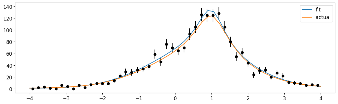
c = cost.ExtendedUnbinnedNLL(xmix, cauchy_on_gauss.pdf_ext)

m = Minuit(c, (xr[0], xr[1], 100, 0.1, 0.1, 0.3, 100, 1, 2))
m.fixed[0, 1] = True  # fix the x_lo, x_hi
m.limits[2, 6] = (0, None)
m.limits[3] = (0, 1)
m.limits[4, 5, 7, 8] = (0, 2)
print(m.migrad())

plt.errorbar(cx, n, n**0.5, fmt="ok")
xm = np.linspace(*xr)
plt.plot(xm, cauchy_on_gauss.pdf_ext(xm, np.array(m.values))[1] * dx[0], label="fit")
plt.legend();
┌─────────────────────────────────────────────────────────────────────────┐
│                                Migrad                                   │
├──────────────────────────────────┬──────────────────────────────────────┤
│ FCN = -1.875e+04                 │              Nfcn = 458              │
│ EDM = 1.58e-05 (Goal: 0.0002)    │            time = 0.1 sec            │
├──────────────────────────────────┼──────────────────────────────────────┤
│          Valid Minimum           │        No Parameters at limit        │
├──────────────────────────────────┼──────────────────────────────────────┤
│ Below EDM threshold (goal x 10)  │           Below call limit           │
├───────────────┬──────────────────┼───────────┬─────────────┬────────────┤
│  Covariance   │     Hesse ok     │APPROXIMATE│NOT pos. def.│   FORCED   │
└───────────────┴──────────────────┴───────────┴─────────────┴────────────┘
┌───┬──────┬───────────┬───────────┬────────────┬────────────┬─────────┬─────────┬───────┐
│   │ Name │   Value   │ Hesse Err │ Minos Err- │ Minos Err+ │ Limit-  │ Limit+  │ Fixed │
├───┼──────┼───────────┼───────────┼────────────┼────────────┼─────────┼─────────┼───────┤
│ 0 │ x0   │   -4.00   │   0.04    │            │            │         │         │  yes  │
│ 1 │ x1   │   4.00    │   0.04    │            │            │         │         │  yes  │
│ 2 │ x2   │   4.4e3   │   2.3e3   │            │            │    0    │         │       │
│ 3 │ x3   │   0.27    │   0.14    │            │            │    0    │    1    │       │
│ 4 │ x4   │   0.57    │   0.06    │            │            │    0    │    2    │       │
│ 5 │ x5   │   1.32    │   0.05    │            │            │    0    │    2    │       │
│ 6 │ x6   │  1.07e3   │  0.27e3   │            │            │    0    │         │       │
│ 7 │ x7   │   0.98    │   0.04    │            │            │    0    │    2    │       │
│ 8 │ x8   │   0.50    │   0.08    │            │            │    0    │    2    │       │
└───┴──────┴───────────┴───────────┴────────────┴────────────┴─────────┴─────────┴───────┘
┌────┬───────────────────────────────────────────────────────────────────────────────────────────┐
│    │        x0        x1        x2        x3        x4        x5        x6        x7        x8 │
├────┼───────────────────────────────────────────────────────────────────────────────────────────┤
│ x0 │         0         0         0         0         0         0         0         0         0 │
│ x1 │         0         0         0         0         0         0         0         0         0 │
│ x2 │         0         0  5.36e+06      -324      5.97      2.36 -5.09e+05         1     -12.5 │
│ x3 │         0         0      -324    0.0204  0.000599  0.000153      26.7  3.53e-05 -0.000986 │
│ x4 │         0         0      5.97  0.000599   0.00384  0.000706     -5.74 -0.000882  -0.00206 │
│ x5 │         0         0      2.36  0.000153  0.000706    0.0021     -1.93 -0.000405  -0.00165 │
│ x6 │         0         0 -5.09e+05      26.7     -5.74     -1.93   7.3e+04    -0.631      11.1 │
│ x7 │         0         0         1  3.53e-05 -0.000882 -0.000405    -0.631   0.00193 -0.000193 │
│ x8 │         0         0     -12.5 -0.000986  -0.00206  -0.00165      11.1 -0.000193   0.00617 │
└────┴───────────────────────────────────────────────────────────────────────────────────────────┘
Let’s see if that last fit agrees with a fit from a function we would define “by hand”#
[40]:
def cauchy_gauss_pdf_ext(x, x_lo, x_hi, A, B, frac, mu, sigma, mu2, sigma2):
    return A * frac * np.diff(
        gaussian.get_cdf(np.array([x_lo, x_hi]), mu, sigma)
    ) + B * (1 - frac) * np.diff(
        cauchy.get_cdf(np.array([x_lo, x_hi]), mu2, sigma2)
    ), A * frac * gaussian.get_pdf(
        x, mu, sigma
    ) + (
        1 - frac
    ) * B * cauchy.get_pdf(
        x, mu2, sigma2
    )
[41]:
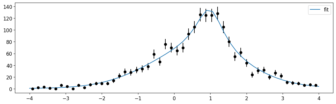
c = cost.ExtendedUnbinnedNLL(xmix, cauchy_gauss_pdf_ext)

m = Minuit(c, xr[0], xr[1], 100, 100, 0.1, 0.1, 0.3, 1, 2)
m.fixed[0, 1] = True  # fix the x_lo, x_hi
m.limits[2, 3] = (0, None)
m.limits[4] = (0, 1)
m.limits[5, 6, 7, 8] = (0, 2)
print(m.migrad())

plt.errorbar(cx, n, n**0.5, fmt="ok")
xm = np.linspace(*xr)
plt.plot(xm, cauchy_gauss_pdf_ext(xm, *m.values)[1] * dx[0], label="fit")
plt.legend();
┌─────────────────────────────────────────────────────────────────────────┐
│                                Migrad                                   │
├──────────────────────────────────┬──────────────────────────────────────┤
│ FCN = -1.875e+04                 │              Nfcn = 458              │
│ EDM = 1.58e-05 (Goal: 0.0002)    │                                      │
├──────────────────────────────────┼──────────────────────────────────────┤
│          Valid Minimum           │        No Parameters at limit        │
├──────────────────────────────────┼──────────────────────────────────────┤
│ Below EDM threshold (goal x 10)  │           Below call limit           │
├───────────────┬──────────────────┼───────────┬─────────────┬────────────┤
│  Covariance   │     Hesse ok     │APPROXIMATE│NOT pos. def.│   FORCED   │
└───────────────┴──────────────────┴───────────┴─────────────┴────────────┘
┌───┬────────┬───────────┬───────────┬────────────┬────────────┬─────────┬─────────┬───────┐
│   │ Name   │   Value   │ Hesse Err │ Minos Err- │ Minos Err+ │ Limit-  │ Limit+  │ Fixed │
├───┼────────┼───────────┼───────────┼────────────┼────────────┼─────────┼─────────┼───────┤
│ 0 │ x_lo   │   -4.00   │   0.04    │            │            │         │         │  yes  │
│ 1 │ x_hi   │   4.00    │   0.04    │            │            │         │         │  yes  │
│ 2 │ A      │   4.4e3   │   2.3e3   │            │            │    0    │         │       │
│ 3 │ B      │  1.07e3   │  0.27e3   │            │            │    0    │         │       │
│ 4 │ frac   │   0.27    │   0.14    │            │            │    0    │    1    │       │
│ 5 │ mu     │   0.57    │   0.06    │            │            │    0    │    2    │       │
│ 6 │ sigma  │   1.32    │   0.05    │            │            │    0    │    2    │       │
│ 7 │ mu2    │   0.98    │   0.04    │            │            │    0    │    2    │       │
│ 8 │ sigma2 │   0.50    │   0.08    │            │            │    0    │    2    │       │
└───┴────────┴───────────┴───────────┴────────────┴────────────┴─────────┴─────────┴───────┘
┌────────┬───────────────────────────────────────────────────────────────────────────────────────────┐
│        │      x_lo      x_hi         A         B      frac        mu     sigma       mu2    sigma2 │
├────────┼───────────────────────────────────────────────────────────────────────────────────────────┤
│   x_lo │         0         0         0         0         0         0         0         0         0 │
│   x_hi │         0         0         0         0         0         0         0         0         0 │
│      A │         0         0  5.36e+06 -5.08e+05      -324      5.96      2.36         1     -12.5 │
│      B │         0         0 -5.08e+05   7.3e+04      26.7     -5.74     -1.93    -0.631      11.1 │
│   frac │         0         0      -324      26.7    0.0204    0.0006  0.000153  3.54e-05 -0.000986 │
│     mu │         0         0      5.96     -5.74    0.0006   0.00384  0.000706 -0.000882  -0.00206 │
│  sigma │         0         0      2.36     -1.93  0.000153  0.000706    0.0021 -0.000405  -0.00165 │
│    mu2 │         0         0         1    -0.631  3.54e-05 -0.000882 -0.000405   0.00193 -0.000193 │
│ sigma2 │         0         0     -12.5      11.1 -0.000986  -0.00206  -0.00165 -0.000193   0.00617 │
└────────┴───────────────────────────────────────────────────────────────────────────────────────────┘

We see that sum_dists reproduces results quickly and without the need for spending time writing new methods for each of the summed distributions.
Conclusion#
Hopefully you have learned how to use the distributions and tools packaged in pygama for your own scientific purposes. If there’s a distribution you see is missing, feel free to contribute it using the conventions described above!
This page has been automatically generated by nbsphinx and can be run as a Jupyter notebook available in the pygama repository.